Workshop 3 Advanced Tree-Based Methods: Bagging, Random Forests and Boosting

In the last workshop, we applied the standard CART to the Boston housing data (modelling variable “medv” using the rest of variables).

library(ISLR)
library(tree)
library(skimr)
library(MASS)

#skim(Boston)
set.seed (180)
train = sample (1: nrow(Boston ), nrow(Boston )/2)
data_train=Boston[train,]
data_test=Boston[-train,]
tree.boston=tree(medv~.,data_train)
summary(tree.boston)

## 
## Regression tree:
## tree(formula = medv ~ ., data = data_train)
## Variables actually used in tree construction:
## [1] "rm"    "lstat" "nox"   "crim" 
## Number of terminal nodes:  7 
## Residual mean deviance:  14.29 = 3516 / 246 
## Distribution of residuals:
##       Min.    1st Qu.     Median       Mean    3rd Qu.       Max. 
## -10.680000  -2.100000  -0.002439   0.000000   1.722000  22.460000

plot(tree.boston)
text(tree.boston,pretty =0)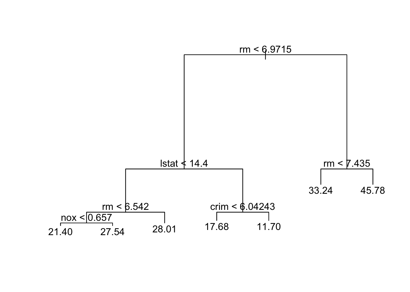

yhat=predict(tree.boston,data_test)
mean((yhat -data_test$medv)^2)

## [1] 27.50751

cv.boston =cv.tree(tree.boston)
plot(cv.boston)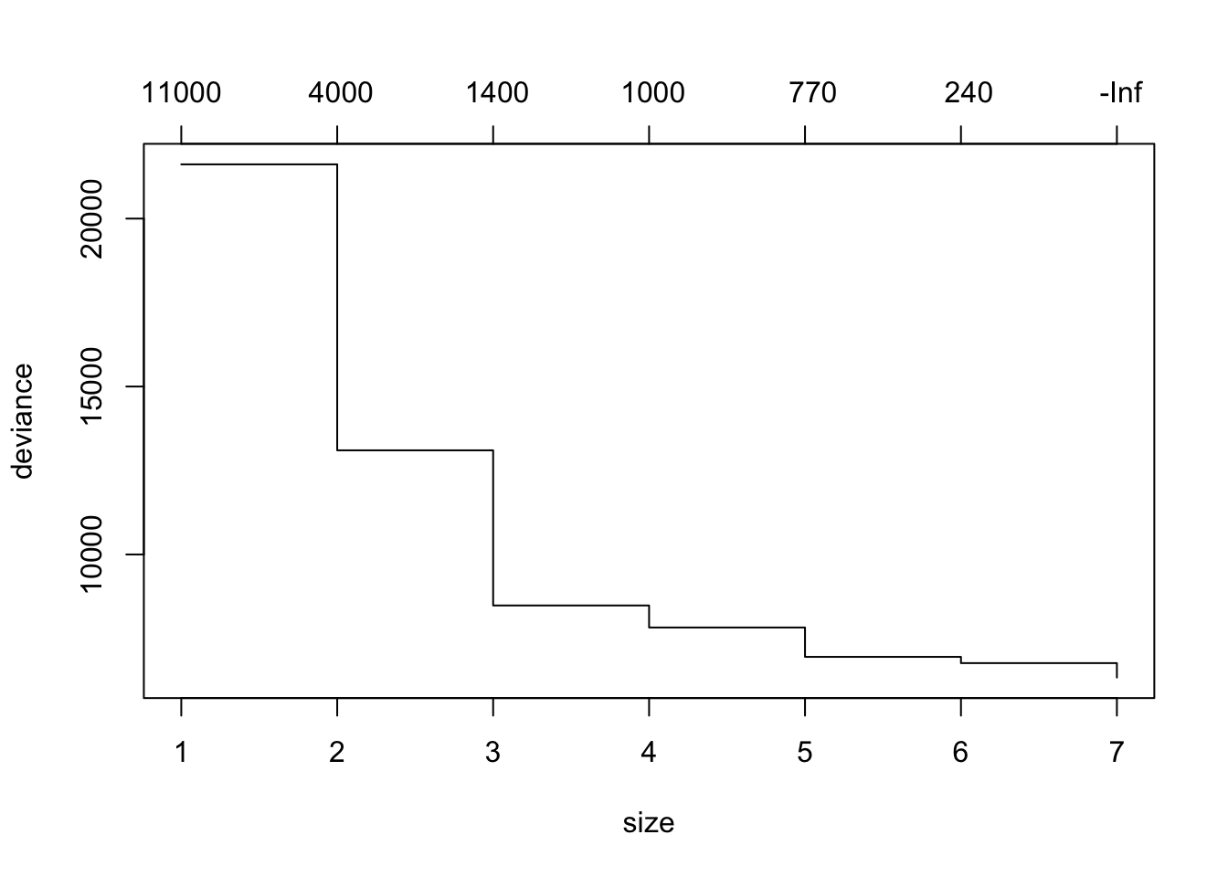

prune.boston =prune.tree(tree.boston ,best =6)
plot(prune.boston)
text(prune.boston,pretty =0)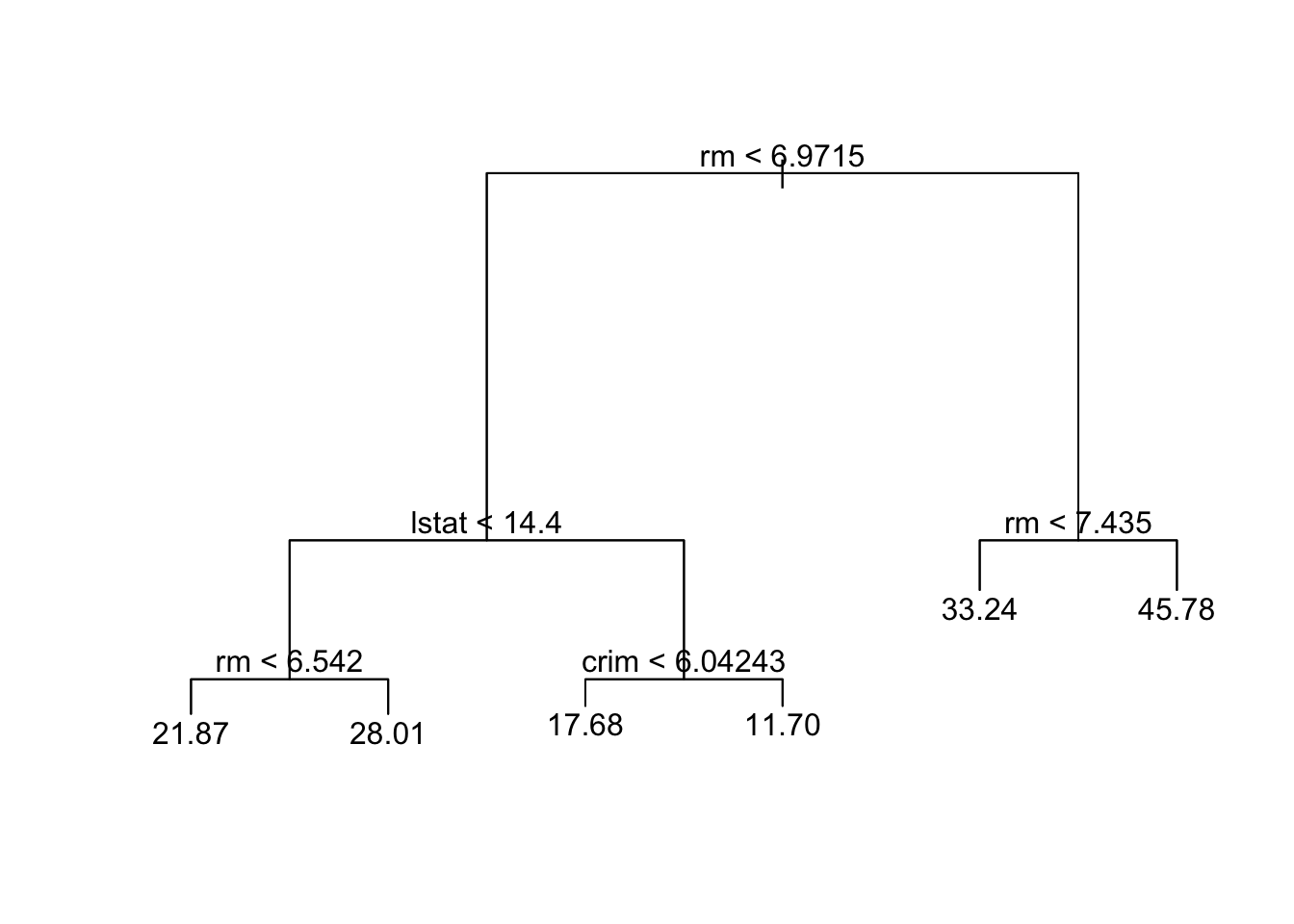

pred.cart=predict(prune.boston,data_test)
mean((pred.cart -data_test$medv)^2)

## [1] 25.61852

========================================================

We now apply bagging and random forests to the Boston data, using the randomForest package in R. Note that bagging is simply a special case of a random forest with m = p. Therefore, the randomForest() function can be used to perform both random forests and bagging. We perform bagging as follows:

library (randomForest)

## randomForest 4.6-14

## Type rfNews() to see new features/changes/bug fixes.

#you may need to install the randomForest library first
set.seed (472)
bag.boston =randomForest(medv~.,data=data_train,mtry=13, ntree=10, importance =TRUE)
bag.boston

## 
## Call:
##  randomForest(formula = medv ~ ., data = data_train, mtry = 13,      ntree = 10, importance = TRUE) 
##                Type of random forest: regression
##                      Number of trees: 10
## No. of variables tried at each split: 13
## 
##           Mean of squared residuals: 21.7334
##                     % Var explained: 74.43

Note there are 13 predictors in the Boston data, the argument mtry=13 indicates that all 13 predictors are considered for each split of the tree, in other words, bagging is conducted. ntree=10 indicates 10 bootstrap trees are generated in this bagged model. The MSR and % variance explained are based on OOB (out-of-bag) estimates

We can also evaluate the performance of bagged model using the test set:

pred.bag = predict (bag.boston,newdata =data_test)
plot(pred.bag , data_test$medv)
abline (0,1)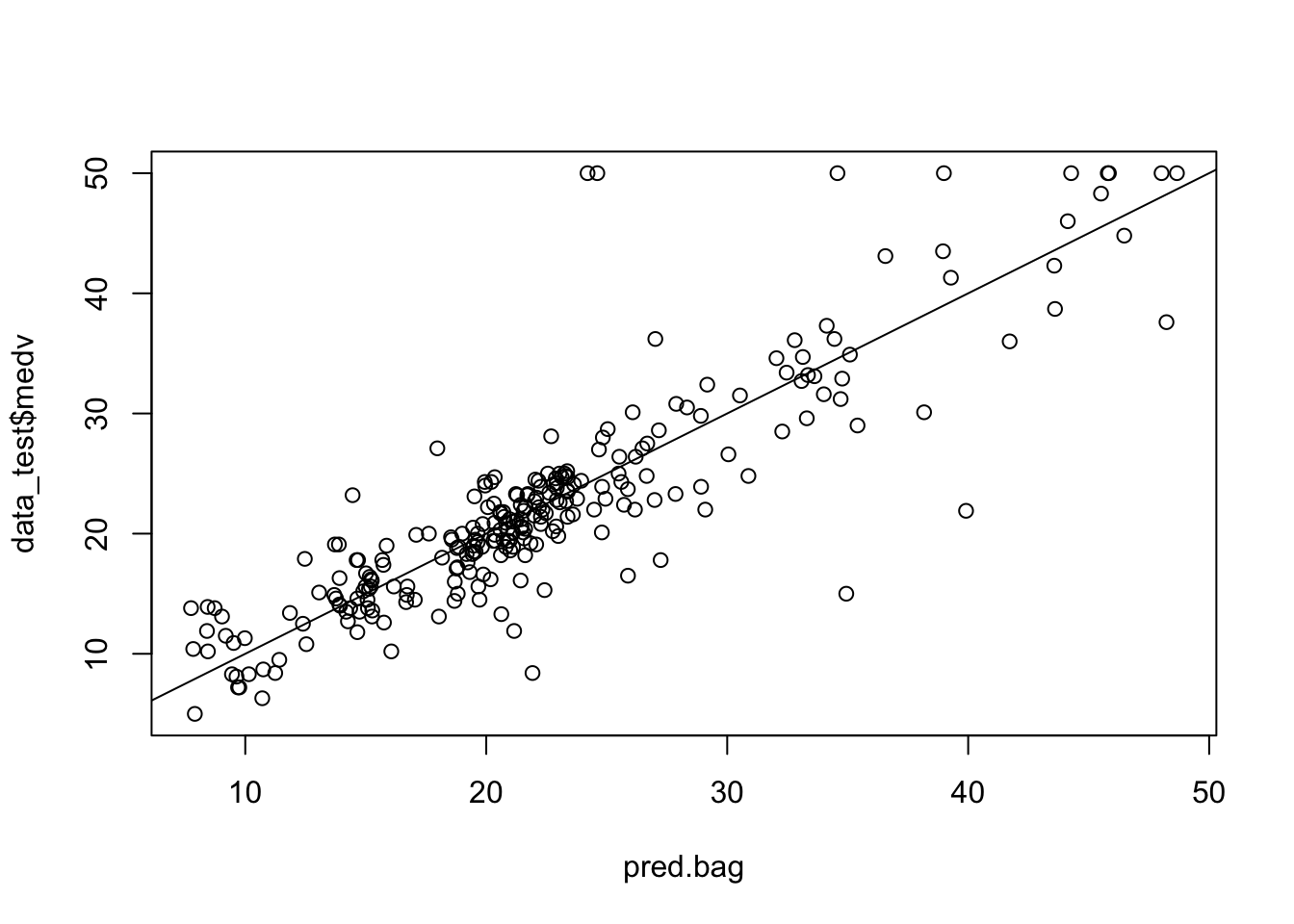

mean(( pred.bag -data_test$medv)^2)

## [1] 19.50244

The test set MSE associated with the bagged regression tree is much smaller than that obtained using an optimally-pruned single CART.

========================================================

Excercise 1.1

   * Increasing the number of bootstrap trees generated in the bagged model to 100 and 1000, record the test set MSE respectively and compare them to the bagged model with 10 bootstrap trees.

========================================================

Random Forests

========================================================

Growing a random forest proceeds in exactly the same way, except that we use a smaller value of the mtry argument. By default, randomForest() uses p/3 variables when building a random forest of regression trees, and sqrt(p) variables when building a random forest of classification trees.

========================================================

Excercise 1.2

   * Build a random forest by considering 4 out of total 13 predictors in each split fitting.
   * Record the test set MSE and compare it with that from bagging.

========================================================

Excercise 1.3

  * Using the importance() function to view the importance of each variable. And interpret the outputs. (hint: type ?importance in the console for detailed description of importance() function) 
  * Using the varImpPlot() to plot the importance measures and interpret the results. (hint: ?varImpPlot).

========================================================

Excercise 1.4

  * write a "for" loop to record the prediction MSE for all 13 possible values of "mtry". (hint: for(mtry_t in 1:13){...})

========================================================

Boosting

========================================================

Here we use the gbm package, and within it the gbm() function, to fit boosted regression trees to the Boston data set.

library (gbm)

## Loaded gbm 2.1.8

set.seed (517)
boost.boston =gbm(medv~.,data=data_train, distribution="gaussian",
n.trees =1000, interaction.depth =2)
summary(boost.boston)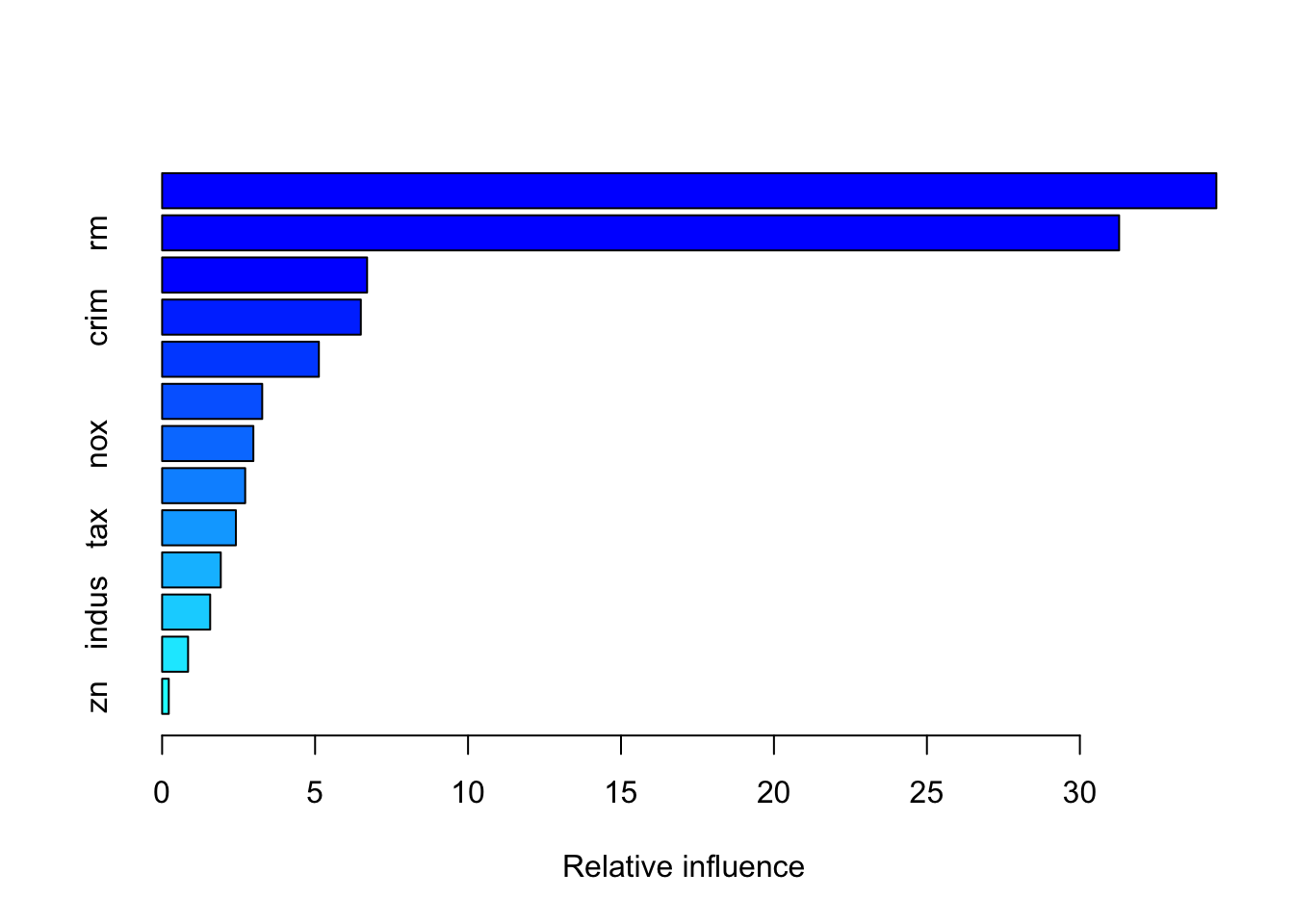

##             var    rel.inf
## lstat     lstat 34.4614597
## rm           rm 31.2829874
## dis         dis  6.7004987
## crim       crim  6.4956378
## black     black  5.1243445
## ptratio ptratio  3.2719527
## nox         nox  2.9828948
## age         age  2.7153448
## tax         tax  2.4112109
## chas       chas  1.9172966
## indus     indus  1.5706205
## rad         rad  0.8485787
## zn           zn  0.2171729

You may look up the function gbm via ?gbm. The option distribution=“gaussian” since this is a regression problem; if it were a binary classification problem, we would use distribution=“bernoulli”. The argument n.trees=1000 indicates that we want 1000 trees, and the option interaction.depth=2 specifies the number of splits performed on each tree. The summary() function produces a relative influence plot and also outputs the relative influence statistics.

We now use the boosted model to predict medv on the test set, and record MSE. Does the boosted model outperfom random forests model built early?

pred.boost=predict(boost.boston,newdata =data_test, n.trees =1000)
mean((pred.boost-data_test$medv)^2)

## [1] 13.54221

The default shrinkage parameter lambda is 0.001. We can specify its value by adding argument shrinkage in the gbm() function, for example shrinkage=0.05.

========================================================

Excercise 1.5

  * Rebuild boosted regression tree model but assign shrinkage parameter to be 0.1.
  * Evaluate the model using the test set and record the MSE to compare with that obtained from former boosted regression tree.
  * Rebuild boosted regression tree model but assign shrinkage parameter to be 0.1 and the number of splits performed on each tree to be 4.
  * Evaluate the model using the test set and record the MSE to compare with that obtained from former boosted regression tree.

========================================================

Now let’s apply what we have learned on a brand new data set, credit_data. The data set set in the modeldata package. It contains a data set from a credit scoring analysis project. Description of the data variable can be found: https://github.com/gastonstat/CreditScoring

library(modeldata)
data(credit_data)
credit_data=na.omit(credit_data)
#There are some missing data in the data set, using na.omit() to remove them.

The goal is to build a model to predict variable “Status” using the rest of variables.

========================================================

Excercise 1.6

Use skim() function to look at the summary of the data
Divide the dataset into two part, training set (half the dataset) and test set (the other half the dataset).
Fit a standard CART tree (with pruning) to the training set, plot the tree
Predict “Status” using the test set and record the classification error
Build an random forest model to the data, evaluate using the test set record the classification error
Build a boosting model to the data, evaluate using the test set record the classification error

========================================================

James, G., Witten D., Hastie T., and Tibshirani R. 2021. An Introduction to Statistical Learning : With Applications in r. New York: Springer.