Workshop 1 Classification and Regression Trees
In this workshop, we will explore the classification and regression trees introduced in the first lecture.
Part I
The first experiment will be based on synthetic (surrogate) datasets. As the name suggests, quite obviously, a synthetic dataset is a repository of data that is generated programmatically (artificially), it is not collected by any real-life survey or experiment. In practice, it is almost impossible to know the underlying system behind the real data. For synthetic data, however, we know exactly what is the underlying system behind the data. It provides a flexible and rich “test” environment to help us to explore a methodology, demonstrate its effectiveness and uncover its pros and cons by conducting experiments upon. For example, if we want to test a linear regression fitting algorithm, we may create a synthetic dataset using a linear regression model and pretend not knowing the parameters of the model.
In the first lecture, we introduced a greedy (top-down) fitting algorithm for building classification and regression tree. Let’s create a synthetic dataset to explore the algorithm.
set.seed(212)
data_surrogate <- data.frame(x = c(runif(200, 0, 0.4), runif(400, 0.4, 0.65), runif(300, 0.65, 1)),
                             y = c(rnorm(200, 1.5), rnorm(400, 0), rnorm(300, 2)))
set.seed() function is used to set the random generator state. So that the random data generated later can be reproduced using the same “seed”. For more information, run ?set.seed in the R console window.
========================================================
Excercise 1.1:
- Please explain how the data frame “data_surrogate” was generated. You may look up the function runif and rnorm via ?runif and ?rnorm.
========================================================
It is always a good idea to plot the data before analysing and modelling it. Here is a visualization of the data set.
plot(x=data_surrogate$x[1:200], y=data_surrogate$y[1:200], col='blue', xlab="X", ylab="Y", pch=19, xlim=c(0,1),ylim=c(-2,4))
points(x=data_surrogate$x[201:600], y=data_surrogate$y[201:600], col='red', pch=19)
points(x=data_surrogate$x[601:900], y=data_surrogate$y[601:900], col='green', pch=19)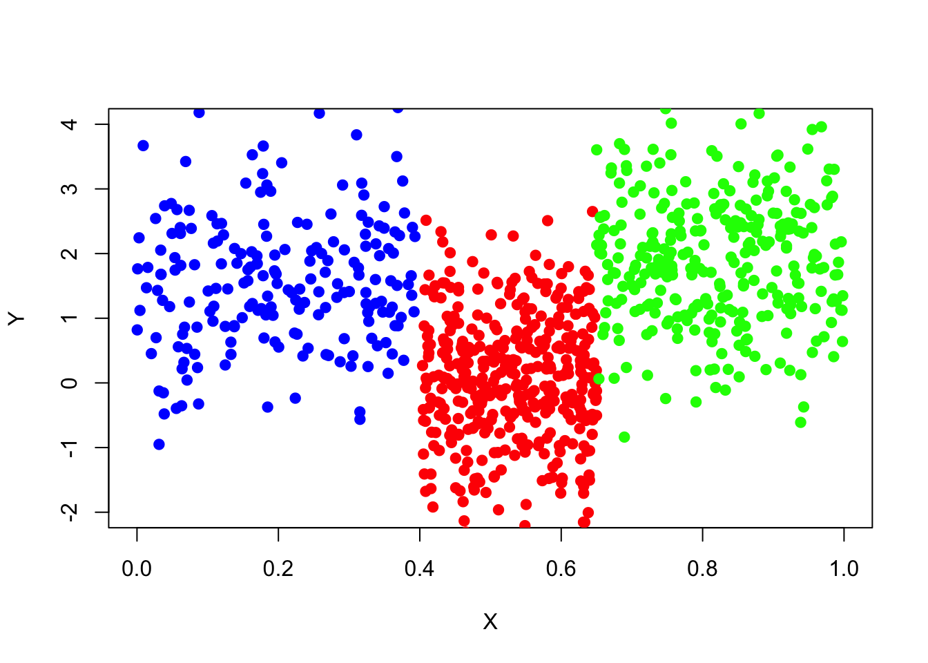
========================================================
Excercise 1.2:
- Now given this data set and knowing how it was generated, what’s the best tree-based model you would expect when modelling variable y using variable x.
========================================================
Now let’s build a regression tree model for this dataset using R.
library("tree")You may need to install the “tree” package first, using install.packages(“tree”).
tree_fit=tree(y~x,data_surrogate)The “tree” function is to fit a classification or regression tree using the greedy fitting algorithm.
summary(tree_fit)##
## Regression tree:
## tree(formula = y ~ x, data = data_surrogate)
## Number of terminal nodes: 3
## Residual mean deviance: 1.001 = 897.9 / 897
## Distribution of residuals:
## Min. 1st Qu. Median Mean 3rd Qu. Max.
## -3.137000 -0.662000 -0.001074 0.000000 0.638100 2.984000#The "summary" function print a summary of the fitted tree object.
tree_fit## node), split, n, deviance, yval
## * denotes terminal node
##
## 1) root 900 1565.0 1.01200
## 2) x < 0.650076 600 883.8 0.55940
## 4) x < 0.398517 200 194.1 1.55700 *
## 5) x > 0.398517 400 391.4 0.06086 *
## 3) x > 0.650076 300 312.4 1.91700 *#print each node as well as the corresponding statisticsThe deviance is simply the residual sum of squares (RSS) for the tree/subtree.
plot(tree_fit)
text(tree_fit,pretty=0)
#If pretty = 0 then the level names of a factor split attributes are used unchanged. This is a nice way to plot the tree model, is it consistent with your previous expectation? Clearly one of the advantages of regression and classification tree model is its interpretation.
After a model is built, do not forget to examine the model performance.
========================================================
Excercise 1.3:
- Create an independent data set (the same way that data_surrogate was created) as a test set, name it data_surrogate_test.
- use “tree_pred=predict(tree_fit,data_surrogate_test)” to generate the model prediction of y variable (in the test set) using the tree model fitted early.
========================================================
========================================================
Exercise 1.4:
- Draw a scatter plot (same as the one drawn for data set “data_surrogate”) for the test set and add the prediction of y, “tree_pred”, to the plot
- Calculate the residual sum of squares.
========================================================
So far everything seems all right! The regression tree works almost perfectly. Note that we have used a rather large data set as a train set to fit the tree, what if the historical data is rather small?
========================================================
Exercise 1.5:
- Create an independent training data set (the same way that data_surrogate was created) but with the number of observations 10 times smaller. And draw a scatter plot of the data.
- Build a regression tree, name “tree_fit_s”, using the new small training set. Look at the summary of the tree model, is it still consistent with your expectation?
- Use the new tree model to predict the y variable in the same test set generated in 1.3 and record the residual sum of squares and compare it with the one you calculated before using the tree model fitted with large training set in 1.4.
Part II
In Part I, We have created an independent small train set and fit a regression tree to it:
set.seed(739)

data_surrogate_s <- data.frame(x = c(runif(20, 0, 0.4), runif(40, 0.4, 0.65), runif(30, 0.65, 1)),
                               y = c(rnorm(20, 1.5),    rnorm(40, 0),         rnorm(30, 2)))

plot(x=data_surrogate_s$x[1:20], y=data_surrogate_s$y[1:20], col='blue', xlab="X", ylab="Y", pch=19, xlim=c(0,1),ylim=c(-2,4))
points(x=data_surrogate_s$x[21:60], y=data_surrogate_s$y[21:60], col='red', pch=19)
points(x=data_surrogate_s$x[61:90], y=data_surrogate_s$y[61:90], col='green', pch=19)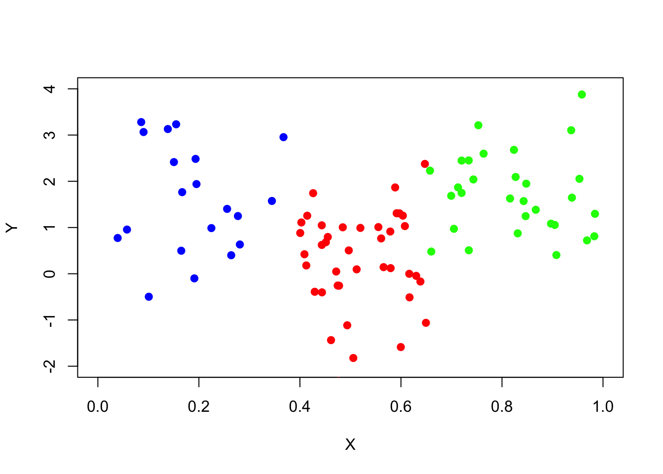
tree_fit_s=tree(y~x,data_surrogate_s)
summary(tree_fit_s)
##
## Regression tree:
## tree(formula = y ~ x, data = data_surrogate_s)
## Number of terminal nodes: 7
## Residual mean deviance: 0.89 = 73.87 / 83
## Distribution of residuals:
## Min. 1st Qu. Median Mean 3rd Qu. Max.
## -2.5420 -0.7364 0.0396 0.0000 0.5973 2.2330tree_fit_s## node), split, n, deviance, yval
## * denotes terminal node
##
## 1) root 90 131.600 1.0660
## 2) x < 0.653469 60 90.670 0.7376
## 4) x < 0.427732 26 29.650 1.4510
## 8) x < 0.160006 8 14.560 2.0450 *
## 9) x > 0.160006 18 11.020 1.1880 *
## 5) x > 0.427732 34 37.640 0.1917
## 10) x < 0.515981 16 15.670 -0.1998
## 20) x < 0.458374 6 1.973 0.3927 *
## 21) x > 0.458374 10 10.330 -0.5554 *
## 11) x > 0.515981 18 17.340 0.5398
## 22) x < 0.59835 9 2.474 0.9361 *
## 23) x > 0.59835 9 12.040 0.1435 *
## 3) x > 0.653469 30 21.480 1.7240 *plot(tree_fit_s)
text(tree_fit_s,pretty=0)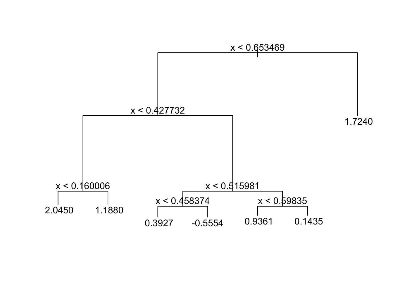
The new fitted tree, “tree_fit_s”, seems to overfit the data, which led to a poor forecast performance in the test set. Now we use the cv.tree() function to see whether pruning the tree using the weakest link algorithm will improve performance.
tree_cv_prune=cv.tree(tree_fit_s,FUN=prune.tree)
tree_cv_prune
## $size
## [1] 7 6 5 4 3 1
##
## $dev
## [1] 127.1730 134.5368 127.4856 127.7807 127.2861 158.3113
##
## $k
## [1] -Inf 2.826888 3.370479 4.065974 4.633948 21.419490
##
## $method
## [1] "deviance"
##
## attr(,"class")
## [1] "prune" "tree.sequence"plot(tree_cv_prune)
Please look up the function cv.tree via ?cv.tree. Note the output k in “tree_cv_prune” is the cost-complexity parameter in the weakest link pruning introduced in the lecture (we used \(\alpha\) in the lecture slides).
tree_fit_prune=prune.tree(tree_fit_s,best=3)
# you may also prune the tree by spefifying the cost-complexity parameter k
# for example tree_fit_prune=prune.tree(tree_fit_s,k=5)
tree_fit_prune
## node), split, n, deviance, yval
## * denotes terminal node
##
## 1) root 90 131.60 1.0660
## 2) x < 0.653469 60 90.67 0.7376
## 4) x < 0.427732 26 29.65 1.4510 *
## 5) x > 0.427732 34 37.64 0.1917 *
## 3) x > 0.653469 30 21.48 1.7240 *plot(tree_fit_prune)
text(tree_fit_prune,pretty=0)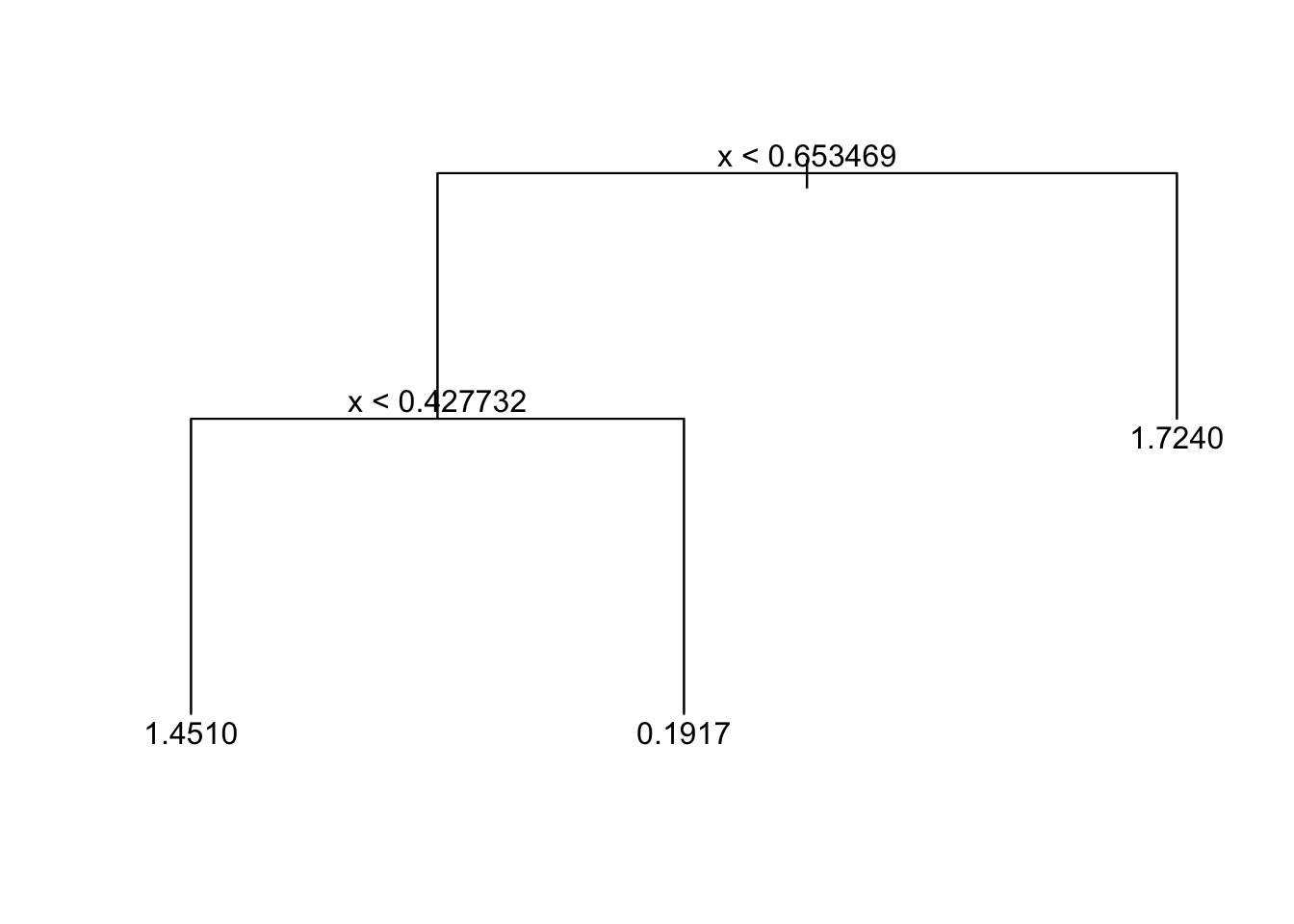
========================================================
Excercise 1.6:
- Use the pruned tree model to predict the y variable in the test set and record the mean squared error.
- Compare the mean squared error with that resulted from unpruned tree
========================================================
========================================================
Excercise 1.7:
- create another small training set, fit regression trees with and without pruning and compare the prediction mean squared error.
========================================================
How would you know that the improved forecast performance is due to pruning rather than the “unlucky” small training set? To demonstrate the robustness of the conclusion, one can conduct the same experiments many times using independent training set.
========================================================
Excercise 1.8:
- create a function named “prune_improvement(k)” that creates an independent small training set and compares pruned and unpruned trees with cost-complexity parameter as input parameter and return the difference in prediction mean squared error.
- run the function 1024 times and calculate the average improvement in prediction mean squared error. You may use “sapply” function, for example: sapply(1:1024, FUN=function(i){prune_improvement(5)})
======================================================== \(~\)