Workshop 2 Classification and Regression Trees continues
In this workshop, we will first explore classification trees by analyzing the Carseats data set.
library(ISLR)
library(tree)
attach(Carseats)
You may need to install the “tree” and “ISLR” package first, using install.packages(“tree”) and install.packages(“ISLR”). “Carseats” is a database in the “ISLR” package, after calling attach(Carseats), objects in the Carseats database can be accessed by simply giving their names.
Please try using “?Carseats” in the console first to read the help notes of the data. First, let’s have a look at the summary of the data using the skimr package. You may need to install the “skimr” package first using install.packages(“skimr”)
library("skimr")
#please try the following code by uncommenting it
#skim(Carseats)
skimr is a great way to get an immediate feel for the data. Please try to run skim(Carseats) and look into the outputs.
In these data, we are interested in how the “Sales” is influenced by the rest of variables. Note that “Sales” is a continuous variable, to build classification tree we first record it as a binary variable. We use the ifelse() function to create a variable, called “High”, which takes on a value of Yes if the Sales variable exceeds 8, and takes on a value of No otherwise. We then include it in the same dataframe via the data.frame() function to merge High with the rest of the Carseats data.
High=ifelse(Sales<=8,"No","Yes")
Carseats=data.frame(Carseats, High)
Carseats$High <- as.factor(Carseats$High)
as.factor() encodes the vector “High” as a factor (categorical variable).
Now we fit a classification tree to these data, and summarize and plot it. Notice that we have to exclude “Sales” from the right-hand side of the formula, because the response is derived from it.
tree.carseats=tree(High~.-Sales,data=Carseats)
summary(tree.carseats)
##
## Classification tree:
## tree(formula = High ~ . - Sales, data = Carseats)
## Variables actually used in tree construction:
## [1] "ShelveLoc" "Price" "Income" "CompPrice" "Population"
## [6] "Advertising" "Age" "US"
## Number of terminal nodes: 27
## Residual mean deviance: 0.4575 = 170.7 / 373
## Misclassification error rate: 0.09 = 36 / 400plot(tree.carseats)
text(tree.carseats,pretty=0)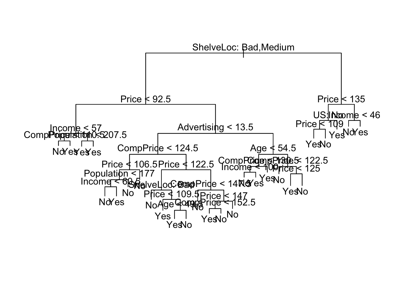
#If pretty = 0 then the level names of a factor split attributes are used unchanged. We see that the training classification error rate is 9%. For classification trees, the deviance is calculated using cross-entropy (see lecture slides).
For a detailed summary of the tree, print it:
tree.carseats## node), split, n, deviance, yval, (yprob)
## * denotes terminal node
##
## 1) root 400 541.500 No ( 0.59000 0.41000 )
## 2) ShelveLoc: Bad,Medium 315 390.600 No ( 0.68889 0.31111 )
## 4) Price < 92.5 46 56.530 Yes ( 0.30435 0.69565 )
## 8) Income < 57 10 12.220 No ( 0.70000 0.30000 )
## 16) CompPrice < 110.5 5 0.000 No ( 1.00000 0.00000 ) *
## 17) CompPrice > 110.5 5 6.730 Yes ( 0.40000 0.60000 ) *
## 9) Income > 57 36 35.470 Yes ( 0.19444 0.80556 )
## 18) Population < 207.5 16 21.170 Yes ( 0.37500 0.62500 ) *
## 19) Population > 207.5 20 7.941 Yes ( 0.05000 0.95000 ) *
## 5) Price > 92.5 269 299.800 No ( 0.75465 0.24535 )
## 10) Advertising < 13.5 224 213.200 No ( 0.81696 0.18304 )
## 20) CompPrice < 124.5 96 44.890 No ( 0.93750 0.06250 )
## 40) Price < 106.5 38 33.150 No ( 0.84211 0.15789 )
## 80) Population < 177 12 16.300 No ( 0.58333 0.41667 )
## 160) Income < 60.5 6 0.000 No ( 1.00000 0.00000 ) *
## 161) Income > 60.5 6 5.407 Yes ( 0.16667 0.83333 ) *
## 81) Population > 177 26 8.477 No ( 0.96154 0.03846 ) *
## 41) Price > 106.5 58 0.000 No ( 1.00000 0.00000 ) *
## 21) CompPrice > 124.5 128 150.200 No ( 0.72656 0.27344 )
## 42) Price < 122.5 51 70.680 Yes ( 0.49020 0.50980 )
## 84) ShelveLoc: Bad 11 6.702 No ( 0.90909 0.09091 ) *
## 85) ShelveLoc: Medium 40 52.930 Yes ( 0.37500 0.62500 )
## 170) Price < 109.5 16 7.481 Yes ( 0.06250 0.93750 ) *
## 171) Price > 109.5 24 32.600 No ( 0.58333 0.41667 )
## 342) Age < 49.5 13 16.050 Yes ( 0.30769 0.69231 ) *
## 343) Age > 49.5 11 6.702 No ( 0.90909 0.09091 ) *
## 43) Price > 122.5 77 55.540 No ( 0.88312 0.11688 )
## 86) CompPrice < 147.5 58 17.400 No ( 0.96552 0.03448 ) *
## 87) CompPrice > 147.5 19 25.010 No ( 0.63158 0.36842 )
## 174) Price < 147 12 16.300 Yes ( 0.41667 0.58333 )
## 348) CompPrice < 152.5 7 5.742 Yes ( 0.14286 0.85714 ) *
## 349) CompPrice > 152.5 5 5.004 No ( 0.80000 0.20000 ) *
## 175) Price > 147 7 0.000 No ( 1.00000 0.00000 ) *
## 11) Advertising > 13.5 45 61.830 Yes ( 0.44444 0.55556 )
## 22) Age < 54.5 25 25.020 Yes ( 0.20000 0.80000 )
## 44) CompPrice < 130.5 14 18.250 Yes ( 0.35714 0.64286 )
## 88) Income < 100 9 12.370 No ( 0.55556 0.44444 ) *
## 89) Income > 100 5 0.000 Yes ( 0.00000 1.00000 ) *
## 45) CompPrice > 130.5 11 0.000 Yes ( 0.00000 1.00000 ) *
## 23) Age > 54.5 20 22.490 No ( 0.75000 0.25000 )
## 46) CompPrice < 122.5 10 0.000 No ( 1.00000 0.00000 ) *
## 47) CompPrice > 122.5 10 13.860 No ( 0.50000 0.50000 )
## 94) Price < 125 5 0.000 Yes ( 0.00000 1.00000 ) *
## 95) Price > 125 5 0.000 No ( 1.00000 0.00000 ) *
## 3) ShelveLoc: Good 85 90.330 Yes ( 0.22353 0.77647 )
## 6) Price < 135 68 49.260 Yes ( 0.11765 0.88235 )
## 12) US: No 17 22.070 Yes ( 0.35294 0.64706 )
## 24) Price < 109 8 0.000 Yes ( 0.00000 1.00000 ) *
## 25) Price > 109 9 11.460 No ( 0.66667 0.33333 ) *
## 13) US: Yes 51 16.880 Yes ( 0.03922 0.96078 ) *
## 7) Price > 135 17 22.070 No ( 0.64706 0.35294 )
## 14) Income < 46 6 0.000 No ( 1.00000 0.00000 ) *
## 15) Income > 46 11 15.160 Yes ( 0.45455 0.54545 ) *In order to properly evaluate the performance of a classification tree on these data, we must estimate the test error rather than simply computing the training error. We split the observations into a training set (250 observations) and a test set (150 observations)
set.seed(926)
train_index=sample(1:nrow(Carseats),250)
data_train=Carseats[train_index,]
data_test=Carseats[-train_index,]
Now we can build a classification tree using the training set, and evaluate its performance on the test set.
tree.carseats=tree(High~.-Sales,data_train)
plot(tree.carseats);text(tree.carseats,pretty=0)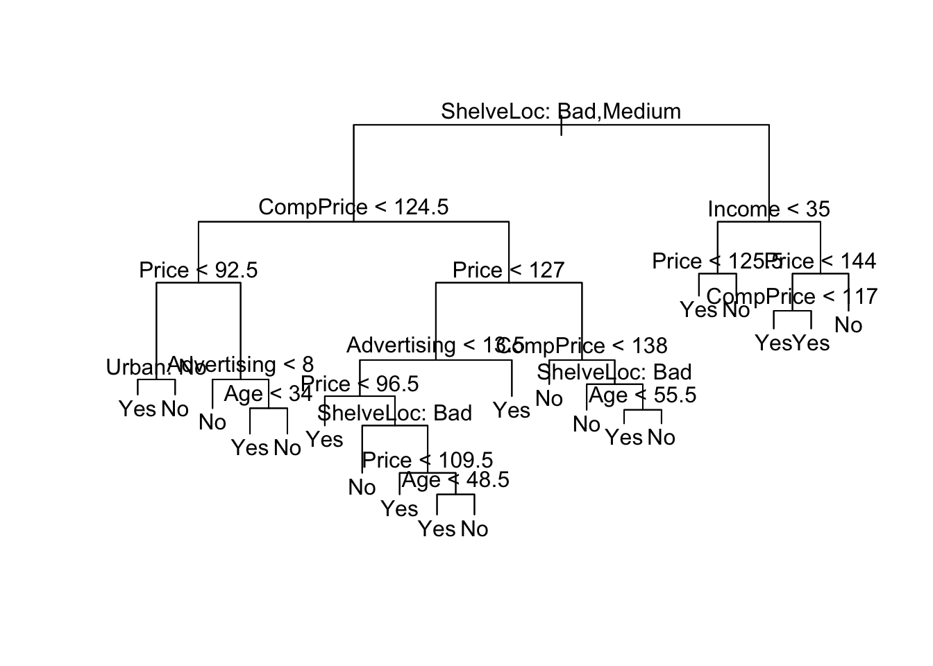
tree.pred=predict(tree.carseats,data_test,type="class")
table(tree.pred, data_test$High)
##
## tree.pred No Yes
## No 70 22
## Yes 16 42========================================================
What is the percentage of correct predictions?
========================================================
This tree was grown to full depth, and might be overfitting. We now use cv.tree to prune it. We use the argument FUN=prune.misclass in order to indicate that we want the classification error rate to guide the cross-validation and pruning process, rather than the default for the cv.tree() function, which is deviance.And we now apply the prune.misclass() function to prune the tree according to the results from cv.tree().
cv.carseats=cv.tree(tree.carseats,FUN=prune.misclass)
cv.carseats
## $size
## [1] 20 19 17 13 11 6 5 4 2 1
##
## $dev
## [1] 61 62 62 64 69 69 74 87 89 102
##
## $k
## [1] -Inf 0.0 0.5 1.0 2.0 3.0 4.0 6.0 8.5 24.0
##
## $method
## [1] "misclass"
##
## attr(,"class")
## [1] "prune" "tree.sequence"plot(cv.carseats)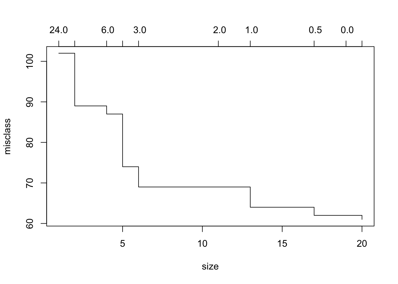
prune.carseats=prune.misclass(tree.carseats,best=10)
plot(prune.carseats);text(prune.carseats,pretty=0)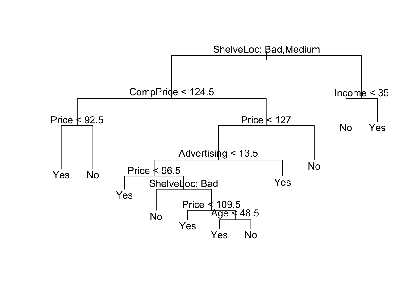
Now lets evaluate this pruned tree on the test data.
tree.pred_prune=predict(prune.carseats,data_test,type="class")
table(tree.pred_prune, data_test$High)
##
## tree.pred_prune No Yes
## No 73 20
## Yes 13 44========================================================
How would you interpret the results comparing with unpruned tree?
========================================================
Now let’s apply what we have learned on a brand new data set, Boston housing data. The data set set in the MASS package. It gives housing values and other statistics in each of 506 suburbs of Boston based on a 1970 census.
library(MASS)The goal is to build a model to predict variable “medv” using the rest of variables.
========================================================
Excercise:
use skim() function to look at the summary of the data
Divide the dataset into two part, training set (half the dataset) and test set (the other half the dataset).
Fit a regression tree to the training set, plot the tree
predict “medv” using the test set and record the mean squared error
prune the tree using cv.tree() and plot the pruned tree
predict “medv” using the test set and pruned tree, recorder the mean squared error and compare it with unpruned tree
comment on your results
========================================================