Chapter 1 Recap and Basic Concepts
1.1 Supervised and Unsupervised Learning
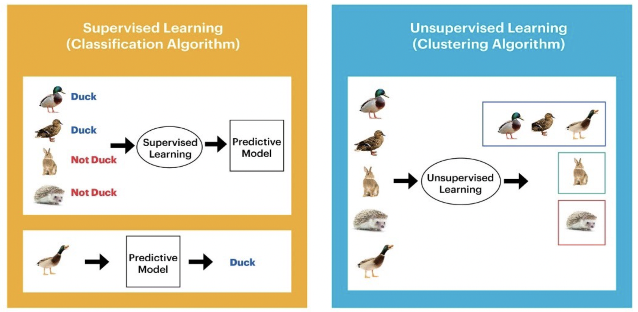
Every machine learning task can be broken down into either supervised learning or unsupervised learning.
Supervised learning involves building a statistical model for predicting or estimating an output based on one or more inputs.
Supervised learning aims to learn a mapping \(f\) from inputs \(\bf{x}\in \mathcal{X}\) to outputs \(\bf{y}\in \mathcal{Y}\). The inputs \(\bf{x}\) are also called the features, covariates, or predictors ; this is often a fixed-dimensional vector of numbers, such as the height and weight of a person, or the pixels in an image. In this case, \(\mathcal{X} = \mathbb{R}^D\) , where \(D\) is the dimensionality of the vector (i.e., the number of input features). The output \(\bf{y}\) is also known as the label , target, or response. In supervised learning, we assume that each input example \(\bf{x}\) in the training archive has an associated set of output targets \(\bf{y}\), and our goal is to learn the input-output mapping \(f\).
The task of Unsupervised learning is to try to “make sense of” data, as opposed to just learning a mapping. That is, we just get observed “inputs” \(\bf{x}\in \mathcal{X}\) without any corresponding “outputs” \(\bf{y}\in \mathcal{Y}\).
From a probabilistic perspective, we can view the task of unsupervised learning as fitting an unconditional model of the form \(p(\bf{x})\), which can generate new data \(\bf{x}\), whereas supervised learning involves fitting a conditional model, \(p(\bf{y}|\bf{x})\), which specifies (a distribution over) outputs given inputs.
Unsupervised learning avoids the need to collect large labelled datasets for training, which can often be time-consuming and expensive (think of asking doctors to label medical images). Unsupervised learning also avoids the need to learn how to partition the world into often arbitrary categories. Finally, unsupervised learning forces the model to “explain” the high-dimensional inputs, rather than just the low-dimensional outputs. This allows us to learn richer models of “how the world works” and discover “interesting structure” in the data.
Here is a simple example that shows the difference between supervised learning and unsupervised learning.
Many classical machine (statistical) learning methods such as linear regression and logistic regression as well as more advanced approaches such as random forests and boosting operate in the supervised learning domain. Most part of this course will be devoted to this setting. For unsupervised learning, we will cover one of the classic linear approaches, principal component analysis, in the first term of the course.
1.2 Classification and Regression
Supervised learning can be further divided into two types of problems: Classification and Regression.
Classification
Classification algorithms are used when the output variable is categorical
The task of the classification algorithm is to find the mapping function to map the input(\(\bf{x}\)) to the discrete output(\(\bf{y}\)).
Example: The best example to understand the Classification problem is Email Spam Detection. The model is trained on the basis of millions of emails on different parameters, and whenever it receives a new email, it identifies whether the email is spam or not. If the email is spam, then it is moved to the Spam folder.
Regression
Regression algorithms are used if there is a relationship between the input variable and the output variable. It is used for the prediction of continuous variables, such as Weather forecasting, Market Trends, etc.
Regression is a process of finding the correlations between dependent and independent variables. It helps in predicting continuous variables such as prediction of Market Trends, prediction of House prices, etc.
The task of the Regression algorithm is to find the mapping function to map the input variable(x) to the continuous output variable(y).
Example: Suppose we want to do weather forecasting, so for this, we will use the Regression algorithm. In weather prediction, the model is trained on past data, and once the training is completed, it can easily predict the weather for future days.
1.3 Parametric vs non-parametric models
Machine learning models can be parametric or non-parametric. Parametric models are those that require the specification of some parameters, while non-parametric models do not rely on any specific parameter settings.
Parametric models
Assumptions about the form of a function can ease the process of machine learning. Parametric models are characterized by the simplification of the function to a known form. A parametric model is a learner that summarizes data through a collection of parameters, \(\bf{\theta}\). These parameters are of a fixed size. This means that the model already knows the number of parameters it requires, regardless of its data.
As an example, let’s look at a simple linear regression model (we will investigate this model thoroughly in the following chapter) in the functional form: \[y=b_0+b_1x+\epsilon\] where \(b_0\) and \(b_1\) are model parameters and \(\epsilon\) reflects the model error. For such a model, feeding in more data will impact the value of the parameters in the equation above. It will not increase the complexity of the model. And note this model form assumes a linear relationship between the input \(x\) and response \(y\).
Non-parametric models
Non-parametric models do not make particular assumptions about the kind of mapping function and do not have a specific form of the mapping function. Therefore they have the freedom to choose any functional form from the training data.
One might think that non-parametric means that there are no parameters. However, this is NOT true. Rather, it simply means that the parameters are (not only) adjustable but can also change. This leads to a key distinction between parametric and non-parametric algorithms. We mentioned that parametric algorithms have a fixed number of parameters, regardless of the amount of training data. However, in the case of non-parametric ones, the number of parameters is dependent on the amount of training data. Usually, the more training data, the greater the number of parameters. A consequence of this is that non-parametric models may take much longer to train.
The classification and regression tree (which will be introduced later in the course) is an example of a non-parametric model. It makes no distributional assumptions on the data and increasing the amount of training data is very likely to increase the complexity of the tree.
1.4 Uncertainty
Arguably, we are living in a deterministic universe without considering quantum theory, which means the underlying system that generates the data is deterministic. One might think that the outcome of rolling dice is purely random. Actually, this is NOT true. If one can observe every related detail including for example the smoothness of the landing surface, the air resistance and the exact direction and velocity of the dice once it left the hand, one shall be able to predict the outcome precisely.
If the underlying system is deterministic, why are we studying machine learning from a probabilistic perspective, for example, we use the form \(p(\bf{y}|\bf{x})\) in supervised learning. The answer is uncertainty. There are two major sources of uncertainty.
Data uncertainty
If there are data involved, there is uncertainty induced by measurement error. You might think that well-made rulers, clocks and thermometers should be trustworthy, and give the right answers. But for every measurement - even the most careful - there is always a margin of “error”. To account for measurement error, we often use a noise model. For example \[ x=\tilde{x}+\eta\] where \(x\) is the observed value, \(\tilde{x}\) reflects the “true” value and \(\eta\) is the noise model, for example assuming \(\eta\sim N(0,1)\).
Model discrepancy
Another major source of uncertainty in modelling is due to model discrepancy. Recall the famous quote from George Box, “All models are wrong, but some models are useful”. There is always a difference between the (imperfect) model used to approximate reality, and reality itself; this difference is termed model discrepancy. Therefore whatever model we construct, we usually include an error term to account for uncertainty due to model discrepancy. For example the \(\epsilon\) in the linear regression model we saw before. And we often assume \(\epsilon\) is a random draw from some distribution. \[y=b_0+b_1x+\epsilon\]
1.5 Model Assessment
Assessment of model performance is extremely important in practice, since it guides the choice of machine learning algorithm or model, and gives us a measure of the quality of the ultimately chosen model.
It is important to note that there are in fact two separate goals here:
Model selection: estimating the performance of different models in order to choose the best one.
Model assessment: having chosen a final model, estimating its prediction error (generalization error) over an independent new data sample.
1.5.1 In-sample vs out-of-sample
If we are in a data-rich situation, the best approach for both problems is to randomly divide the dataset into three parts: a training set, a validation/evaluation set, and a test set.
- The training set is used to fit the model parameters.
- The validation set is used to estimate prediction error for model selection (including choosing the values of hyperparameters).
- The test set is used for assessment of the generalization error (also referred to as test error, is the prediction error over an independent test sample.) of the final chosen model.
The period that the training set and the validation set are used for the initial parameter estimation and model selection, is called in-sample period. And an out-of-sample period uses a test set to evaluate final forecasting performance.
Ideally, the test set should be kept in a “vault” and be brought out only at the end of the data analysis. Suppose instead that we use the test set repeatedly, choosing the model with the smallest test-set error. Then the test set error of the final chosen model will underestimate the true test error, sometimes substantially.
It is difficult to give a general rule on how to choose the number of observations in each of the three parts. A typical split might be \(50\%\) for training, and \(25\%\) each for validation and testing.

1.5.2 Cross-Validation
For the situations where there is insufficient data to split it into three parts. One could conduct k-fold Cross-validation on a single training set for both training and validation.
k-fold Cross-validation (CV) involves randomly dividing the set of \(n\) observations into \(k\) groups (or folds) of approximately equal size.
Then, for each group \(i=1,...,k\):
- Fold \(i\) is treated as a validation set, and the model is fit on the remaining \(k-1\) folds.
- The performance metric, \(Performance_i\) (for example MSE), is then computed based on the observations of the held out fold \(i\).
This process results in \(k\) estimates of the test performance, \(Performance_1,...,Performance_k\). The \(k\)-fold CV estimate is computed by averaging these values. \[CV_{(k)} = \frac{1}{k} \sum_{i=1}^{k} Performance_i \]
Figure 1.1 illustrates this nicely.
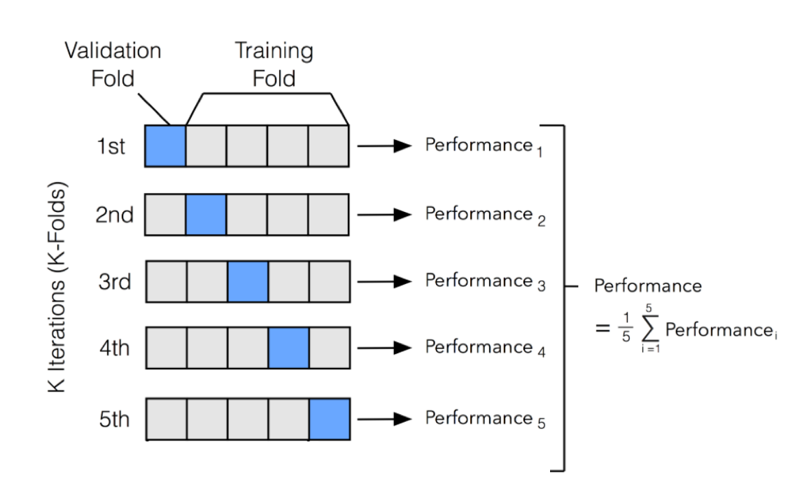
Figure 1.1: An illustration of k-fold CV with 5 folds.
The \(CV_{(k)}\) as an estimate of the test performance can also be used for model selection. Note that to assess the performance of the final chosen model, one still need another independent test sample.
1.5.3 Overfitting vs Underfitting
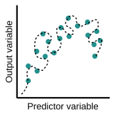
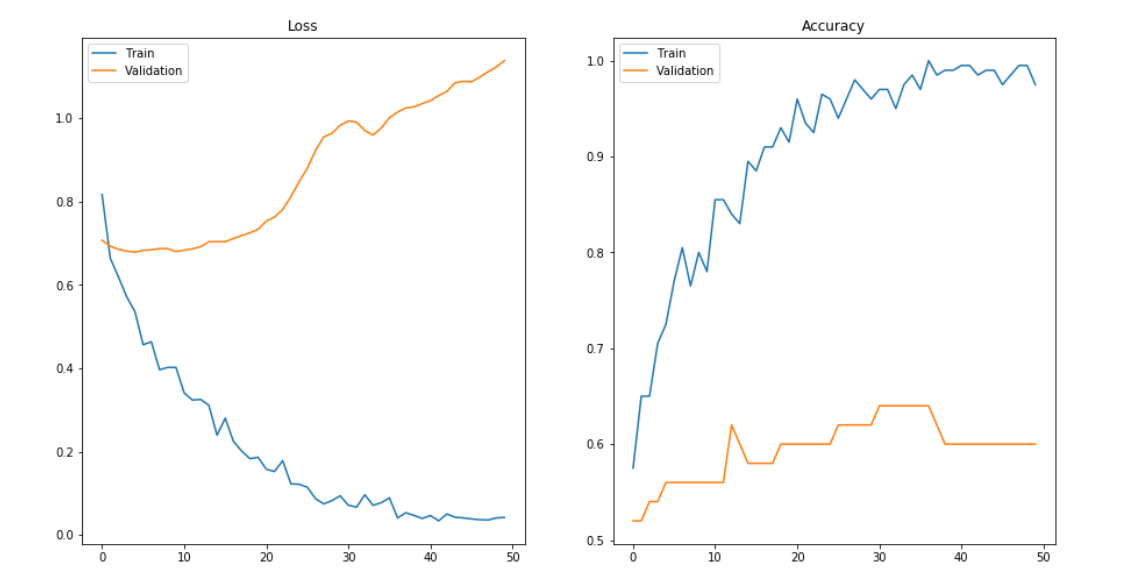
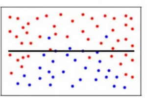
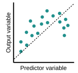
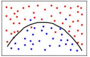
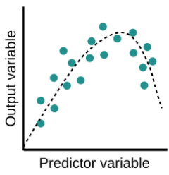
Overfitting is a common pitfall in machine learning modelling, in which a model tries to fit the training data entirely and ends up “memorizing” the data patterns and the noise/random fluctuations. These models fail to generalize and perform well in the case of unseen data scenarios, defeating the model’s purpose. That is why an overfit model results in poor test accuracy. Example of overfitting situation in classification and regression:
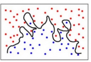
 Detecting overfitting is only possible once we move out of the training phase, for example evaluate the model performance using the validation set.
Underfitting is another common pitfall in machine learning modelling, where the model cannot create a mapping between the input and the target variable that reflects the underlying system, for example due to under-observing the features. Underfitting often leads to a higher error in the training and unseen data samples.
Example of overfitting situation in classification and regression:
Underfitting becomes obvious when the model is too simple and cannot represent a relationship between the input and the output. It is detected when the training error is very high and the model is unable to learn from the training data.
1.5.4 Bias Variance Trade-off
In supervised learning, the model performance can help us to identify or even quantify overfitting/underfitting. Often we use the difference between the actual values and predicted values to evaluate the model, such prediction error can in fact be decomposed into three parts:
- Bias: The difference between the average prediction of our model and the correct value which we are trying to predict. A model with high bias pays very little attention to the training data and oversimplifies the model. It always leads to high error on training and test data.
- Variance: Variance is the variability of model prediction for a given data point or a value which tells us how uncertain our model is. A model with high variance pays a lot of attention to training data and does not generalize on the data which it hasn’t seen before. As a result, such models perform very well on training data but have high error rates on test data.
- Noise: Irreducible error that we cannot eliminate.
Mathematically, assume the relationship between the response \(Y\) and the predictors \(\boldsymbol{X}=(X_1,...,X_p)\) can be represented as:
\[ Y=f(\boldsymbol{X})+\epsilon \] where \(f\) is some fixed but unknown function of \(\boldsymbol{X}\) and \(\epsilon\) is a random error term, which is independent of \(\boldsymbol{X}\) and has mean zero.
Consider building a model \(\hat{f}(\boldsymbol{X})\) of \(f(\boldsymbol{X})\) (for example a linear regression model), the expected squared error (MSE) at a point x is
\[\begin{equation} \begin{split} MSE & = E\left[\left(y-\hat{f}(x)\right)^2\right]\\ & = E\left[\left(f(x)+\epsilon-\hat{f}(x)\right)^2\right] \\ & = E\left[\left(f(x)+\epsilon-\hat{f}(x)+E[\hat{f}(x)]-E[\hat{f}(x)]\right)^2\right] \\ & = ... \\ & = \left(f(x)-E[\hat{f}(x)]\right)^2+E\left[\epsilon^2\right]+E\left[\left(E[\hat{f}(x)]-\hat{f}(x)\right)^2\right] \\ & = \left(f(x)-E[\hat{f}(x)]\right)^2+Var[\epsilon]+Var\left[\hat{f}(x)\right]\\ & = Bias[\hat{f}(x)]^2+Var[\epsilon]+Var\left[\hat{f}(x)\right]\\ & = Bias^2+Variance+Irreducible\; Error \end{split} \end{equation}\]
We can create a graphical visualization of bias and variance using a bulls-eye diagram. Imagine that the center of the target is a model that perfectly predicts the correct values. As we move away from the bulls-eye, our predictions get worse and worse.
We can plot four different cases representing combinations of both high and low bias and variance.
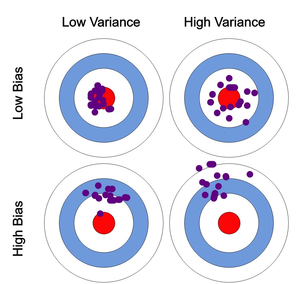
At its root, dealing with bias and variance is really about dealing with overfitting and underfitting. High bias and low variance are the most common indicators of underfitting. Similarly, low bias and high variance are the most common indicators of overfitting. Bias is reduced and variance is increased in relation to model complexity. As more and more parameters are added to a model, the complexity of the model rises and variance becomes our primary concern while bias steadily falls.
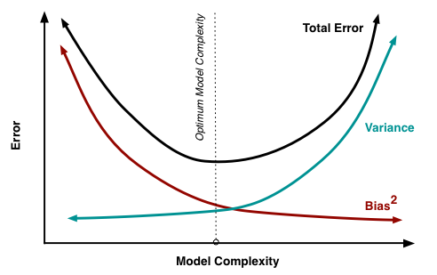
An optimal balance of bias and variance would neither overfit nor underfit the model.
Example of an optimal balanced situation in classification and regression:
1.6 What do we need?
What do we need to achieve “successful” Machine (Statistical) Learning? In my opinion, it requires the following four pillars.
1. Sufficient Data
If you ask any data scientist how much data is needed for machine learning, you’ll most probably get either “It depends” or “The more, the better.” And the thing is, both answers are correct.
It really depends on the type of project you’re working on, and it’s always a great idea to have as many relevant and reliable examples in the datasets as you can get to receive accurate results. But the question remains: how much is enough?
General speaking, more complex algorithms always require a larger amount of data. The more features (the number of input parameters), model parameters, and variability of the expected output it should take into account, the more data you need. For example, you want to train the model to predict housing prices. You are given a table where each row is a house, and the columns are the location, the neighborhood, the number of bedrooms, floors, bathrooms, etc., and the price. In this case, you train the model to predict prices based on the change of variables in the columns. And to learn how each additional input feature influences the input, you’ll need more data examples.
2. Sufficient Computational Resources
There are four steps for conducting machine learning, all require sufficient computational resources:
- Preprocessing input data
- Training the machine learning model
- Storing the trained machine learning model
- Deployment of the model
Among all these, training the machine learning model is the most computationally intensive task. For example, training a neural network often requires intensive computational resources to conduct an enormous amount of matrix multiplications.
3. Performance metrics
Performance metrics are a part of every machine learning pipeline. They tell you if you’re making progress, and put a number on it. All machine learning models, whether it’s linear regression or neural networks, need a metric to judge performance.
Many of the machine learning tasks can be broken down into either Regression or Classification. There are dozens of metrics for both problems, for example, Root Mean Squared Error for Regression problem and Accuracy for Classification problem. Choosing a “proper” performance could be crucial to the whole machine learning process. We must carefully choose the metrics for evaluating machine learning performance because
How the performance of ML algorithms is measured and compared will be dependent entirely on the metric you choose.
How you weigh the importance of various characteristics in the result will be influenced completely by the metric you choose.
We will explore some of the popular performance metrics for machine learning in the coming lectures.
Note most of the performance metrics (especially in supervised learning) require verification/labelled data. For regression problems, we usually require an observed response variable (verification) in order to calculate performance metrics. And for the classification problems, we usually require labelled data. In machine learning, data labelling is the process of identifying raw data (images, text files, videos, etc.) and adding one or more meaningful and informative labels to provide context so that a machine learning model can learn from it. For example, labels might indicate whether a photo contains a bird or car, which words were uttered in an audio recording, or if an x-ray contains a tumor.
4. Proper Machine Learning Algorithm
There are so many algorithms that it can feel overwhelming when algorithm names are thrown around. In this course, we will look into some classic machine learning algorithms including for example linear models, tree-based models and neural networks. Knowing where the algorithms fit is much more important than knowing how to apply them. For example, applying a linear model to the data generated by a nonlinear underlying system is obviously not a good idea.
1.7 Models learned so far
You have explored a number of regression models in the past few months, for example
Linear regression: one of the simplest models that explores the linear relationship between the response and predictors.
Polynomial regression: is introduced to explore the nonlinear relationship between the response and predictors (with the models remaining linear in the parameters). Because the polynomial regression is a global fitting approach, it is rather difficult to reflect local information.
Step functions: is introduced to use cut-points (knots) to fit models locally instead, yet it lacks smoothness.
Splines: is introduced to fit local polynomial regression models in a “smooth” way.
General Additive model: Splines and step functions are designed for single predictor scenarios, GAM is introduced to deal with multiple predictors by adding different single predictor models together. Additivity is convenient, but it is also one of the main limitations of GAMs, which might miss non-linear interactions among predictors.