Chapter 3 Neural Networks and Deep Learning
3.1 Motivation
We are currently living in a data-driven world, where the amount of digitally-collected data grows exponentially. Being a powerful tool, deep learning derives insights from this tremendous amount of data and helps solve many practical problems. Actually, deep learning is a subfield of machine learning, and neural networks make up the backbone of deep learning algorithms.
People who are exploring deep learning as a field to shift their careers or people who are just curious about why there is such a buzz of deep learning all over the places often have one burning question in their mind – what all possible things can one achieve with deep learning? Well, the short answer is – that the possibility is endless and one’s creativity is the only limit.
Here are a few deep learning examples that are in popular use in today’s world.
Deep Learning is an integral part of our daily life
Google search engine, now processes over 40,000 searches per second on average and billions of searches daily and yet throws relevant search results within seconds. Did you ever freak out at how Google gives such accurate autocomplete prompts in the search boxes as if it is reading our minds about search context?
Google maps predict which route will be faster and show such an accurate ETA of reaching the destination.
Ever noticed that spam/junk folder in your university mailbox or many other email providers, for example Gmail, and did you ever open it to see so many spam emails indeed.
Various language translators and automatic subtitles are becoming better and better with time.
Youtube and Tiktok suggestions, which keep people hooked for endless hours. Amazon and Netflix are so good at recommending what you may like.
Yes, I think you are getting my point now, it is deep learning that is behind all the magic.
Deep Learning in industrial uses
Industries are adopting deep learning across the world.
Banks are using deep learning to detect fraud, pass loans, and maintain investment portfolios.
Hospitals are using deep learning to detect and diagnose diseases with more accuracy than actual doctors.
Companies are running ad campaigns targeted to specific customer segments and managing their supply chain and inventory control using deep learning.
Enterprise chatbots are now the next big thing, with companies adopting them to interface with customers.
Online retailers are building their recommendation systems with more accuracy than before using the latest advancements in deep learning.
Self Driving Cars are the latest fascination that has caught the imaginations of companies like Google, Uber, and Tesla who are investing heavily into this future vision using next-generation deep learning technology.
These are just a few of the popular use cases and are just the tip of the iceberg. Deep learning can be used in the most creative ways to solve social, economic, and business problems. The possibility just endless.
Deep Learning – The Artist
This is the coolest part- with so many advancements in Deep Learning a subset field with deep learning things are getting to the next level of reality. Now we are able to produce artwork using deep learning. These are some of the astonishing artworks.
Deepfakes
Jason Allen, a video game designer in Pueblo, Colorado, spent roughly 80 hours working on his entry to the Colorado State Fair’s digital arts competition. Judges awarded his A.I.-generated work (“Théâtre D’opéra Spatial”) first place, which came with a $300 prize.

The beautiful model-looking faces below do not exist and have been generated by deep learning’s imagination.

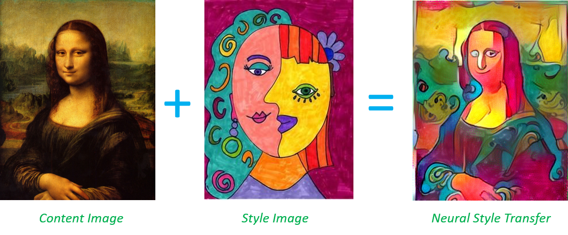
Neural Style Transfer
Neural style transfer is a cool technique in which a style of an image or artwork is transferred to another image.
Music Composer
Nowadays, Deep Learning based apps (for example https://www.aiva.ai/) can assist you in creating various styles of AI-generated music.
Check out this soundtrack music (https://www.youtube.com/watch?v=Emidxpkyk6o&ab_channel=Aiva), there is no reason to believe that it was not generated by humans!!

Deep Learning – The Gamer
In 2011, IBM’s deep learning system Watson participated in a popular TV game show Jeopardy – which competed and defeated the world’s best Jeopardy human champions.
In 2016, Deepmind’s deep learning system AlphaGo played Go with Lee Sudol (the best player and champion of Go) and defeated him. This feat is considered to be one of the greatest achievements in the field of deep learning.
Deep learning-based AI-player has been outcompeting top human players in various real-time strategy games, such as StarCraft and League of Legends.
3.2 Warm up
Deep learning is now an enormous area of study. We have only a week to dip in and sample the wonders! It has taken off in the past few years. Neural networks have been around for ages, but we only recently have the tools, data and computational power to be able to fit many layers deep.
A brief history of deep learning can be found: https://machinelearningknowledge.ai/brief-history-of-deep-learning/
Standard machine (statistical) learning is great for structured data classification and regression, for example when the underlying system is “LINEAR”. Deep learning excels at unstructured (unknown structured), temporal (time series), and image problems, especially when the underlying system is very “NONLINEAR”.
There are some attractive practical reasons for success:
Everything in deep learning boils down to half a dozen tensor (defined later in this session) operations (linear algebra).
Deep learning is very flexible and complex models can be assembled like LEGO.
Explosion in parallel computing and amenability of deep learning to parallelism.
On-line and update learning capabilities of deep learning. (live feeding information)
A “fast” operational model once it is trained.
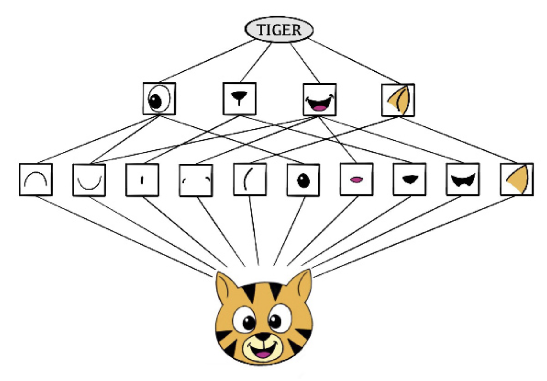
Although Deep Learning is shiny and exciting, we are still in the very early stages of having any theory to understand Deep Learning in particular. Intuitively Deep Learning is learning representations/features from the data without being “taught”. For example, as shown in the figure (James et al. (2021)) below, to identify a tiger from an image, deep learning learns to extract “features” including for example eyes and ears.
Tensors
Tensors are a type of data structure commonly used in deep learning, and like vectors and matrices, you can calculate arithmetic operations with tensors. To slightly oversimplify, a tensor is a generalisation of a vector or matrix.
- Rank-0 tensor: a scalar (just a number!)
- Rank-1 tensor: a vector (c(1,2,3)).
- Rank-2 tensor: a matrix (matrix(…)).
- Rank-3+ tensor: an array (array(…)), multi-dimensional array.
There are well-defined ways of transforming and interacting tensors with each other. All deep learning models boil down to bolting together lots of tensors in a special way.
So far, all the data we have seen has been in matrix form. These are rank-2 or 2D tensors. Some typical data that we encounter in full tensor form include:
- Standard structured data: 2D tensor (obs × features)
- Time series: 3D tensor (obs × time × features)
- Pictures: 4D tensor (obs × vertical × horizontal × RGB colour)
- Video: 5D tensor (obs × time × vertical × horizontal × RGB colour)
Natively working on tensors allows deep learning to account for spatio-temporal locality in a way that is not naturally expressible in classical machine learning.
3.3 Feedforward Neural Networks
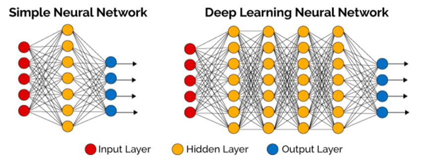
First, let’s explore the classical feedforward neural networks, often referred to as multi-layer perceptrons (MLP) or dense neural networks, referring to the sole use of dense layers in these networks (as opposed to e.g., convolutional layers).
A classic feedforward neural network consists of an input layer, hidden layer(s) and an output layer.
Input Layer Input data is fed into each input neuron in the input layer feature-by-feature. Generally, the input features are not ‘engineered’ in any way, but fed directly to the input layer except for categorical data, one-hot encoding is usually applied to transform categorical variables into binary variables. In the “color” variable example, there are three categories, and, therefore, three binary variables are needed. A “1” value is placed in the binary variable for the color and “0” values for the other colors. It is also normal to either centre and scale the data to mean 0, standard deviation 1; or to map the input to the interval \([0,1]\).
Hidden Layer(s) The input layer first feeds forward to the first hidden layer using the following equation, \[h_i=f(c_i+\sum_j w_{ji}x_j)\] where \(h_i\) is the \(i^{th}\) neuron in the first hidden layer, \(x_j\) is the \(j^{th}\) feature in the input layer, \(c_i\) is the intercept (also called bias), \(w_{ji}\) is the weight (coefficient) and \(f(\cdot)\) is the activation function. Therefore, each neuron in the hidden layer is obtained by applying an activation function \(f\) to a linear combination of all input features. We can extend this formula to allow more than one hidden layer. Often, the activation function is the same for each layer (but need not be). Note that if \(f(\cdot)\) is an activation function, i.e. \(f(z)=z\), we will end up with purely linear networks and won’t be able to learn any non-linear “features”. The preferred choice in modern neural networks is the ReLU (rectified linear ReLU unit) activation function, which takes the form \[f(z)=max\{0,z\}\]
Output layer The last hidden layer feeds forward to produce the output layer. For the regression problem, the output is simply the linear combination of all neurons in the last hidden layer. And for the classification problem, we need to apply the \(sigmoid\) activation function, \[f(z)=\frac{1}{1+e^{-z}}\], which is the same function used in logistic regression to convert a linear function into probabilities.
We of course are interested in the statistical setting where there may be irreducible error, so the model is completed as for other machine (statistical) learning models:
- Regression: \(Y|X\sim N(u=\hat{y},\sigma^2)\)
- Classification: \(Y|X\sim Categorical(\hat{p})\) where \(\hat{y}\) or \(\hat{p}\) are the output of the deep neural network. We, therefore, want the neural network to make a function approximation for the reducible error part of the model. In principle, it is then a straightforward application of maximum likelihood, or the problem of optimisation to find the minimum of the equivalent loss/error function (the negative log-likelihood, ie MSE or cross entropy respectively above).
One of the most striking facts about neural networks is that they can compute any function at all, which comes from the Universal Approximation Theorem. The simplified statement of the Theorem is:
A feedforward network with:
- a linear output layer,
- at least one hidden layer (original theorem was 1 layer),
- any “squashing” activation function (e.g. sigmoid),
can approximate any Borel measurable function from one finite-dimensional space to another with any desired nonzero amount of error, provided that the network is given enough hidden units. In other words, neural networks are provably universal function approximators! See http://neuralnetworksanddeeplearning.com/chap4.html for visual proof that neural nets can compute any function.
The universal approximation theorem guarantees that our deep net is theoretically able to represent the arbitrarily complex relationship between features and response. But,
- we have no results on how big that network should be;
- we have no such guarantee we can learn the parameters of that network;
- we have no guarantees we won’t overfit the data.
We have \(existence\), but no constructive proof that really helps.
To proceed with finding the MLE of some fixed network design, we need to adopt some kind of gradient-based optimiser. But we need to address the following problems:
- What is the gradient of this huge deep neural network?
- How do we find the optimum of this potentially highly non-convex likelihood surface?
- Should we even be trying to find the absolute optimum?
- How can we build in robustness against overfitting?
We will tackle these problems in the following sessions.
3.4 Gradient Descent Optimization
Motivation
Recall that to build linear regression model, \(\bf{Y}=\beta\bf{X}+\bf{\epsilon}\), we need to find “optimal” values of \(\bf{\beta}\). Under the “linear” assumptions, we use Least Squares Fit to estimate \(\bf{\beta}\). Note, this essentially is an optimization problem, i.e find “optimal” estimate of \(\bf{\beta}\) that gives the smallest Least Squares. Similarly, building a neural network model, \(\bf{Y}=Model_{nn}(\bf{X}, \bf{c},W,...)+\bf{\epsilon}\), is also an optimization problem, i.e. find “optimal” estimations of parameters \(\hat{\bf{c}},\hat{W},...\) according to some Loss function. For linear regression, we can find analytical solution of the “optimal” estimates, i.e. \(\hat{\beta}=(\bf{X}^T\bf{X})^{-1}\bf{X}^TY\). When the model is complex, for example the neural networks \(\bf{Y}=Model_{nn}(\bf{X}, \bf{c},W,...)+\bf{\epsilon}\), we need to use some empirical optimization algorithm, for example the classic Gradient Descent Algorithm.
Gradient Descent Algorithm
Consider a Loss function \(\mathcal{L}\) is a convex function of parameters, \(\boldsymbol{\theta}\). To solve the optimization problem, i.e. finding values of the vector of parameters that gives the minimum of the Loss function, \(\boldsymbol{\theta}^*=argmin_{\boldsymbol{\theta}}\mathcal{L}(\boldsymbol{\theta})\). Mathematically, we may solve this problem by solving \(\nabla \mathcal{L} =0\). When the Loss function is formed from a complex model, for example the deep neural networks, we have to solve the problem empirically.
From the simple approximation of the first derivative, we have \(\Delta \mathcal{L} \approx \nabla \mathcal{L} \cdot \Delta \boldsymbol{\theta}\). The idea of the empirical optimization approach is to search the solution iteratively, i.e. update \(\boldsymbol{\theta}\) iteratively with \(\boldsymbol{\theta}'\) that leads to \(\nabla \mathcal{L}\leq0\). If we let \(\Delta \boldsymbol{\theta}=-\alpha \nabla \mathcal{L}\) where \(\alpha>0\), we can guarantee \(\nabla \mathcal{L}\leq0\) as \(\Delta \mathcal{L} \approx -\alpha \nabla \mathcal{L} \cdot \nabla \mathcal{L}=-\alpha \parallel \nabla \mathcal{L} \parallel ^2\leq 0\). Therefore if we keep update \(\boldsymbol{\theta}\) by: \(\boldsymbol{\theta} \rightarrow \boldsymbol{\theta}'=\boldsymbol{\theta}-\gamma \nabla \mathcal{L}\), it will lead us to \(\nabla \mathcal{L}\rightarrow 0\) and \(\mathcal{L}\rightarrow min(\mathcal{L})\). This leads to the Gradient Descent Algorithm.
Gradient Descent Algorithm iteratively calculates the next point using gradient at the current position, scales it (by a learning rate \(\gamma\)) and subtracts obtained value from the current position (makes a step). It subtracts the value because we want to minimise the function (to maximise it would be adding). This process can be written as: \[\boldsymbol{\theta}^{i+1}=\boldsymbol{\theta}^{i}-\gamma \nabla \mathcal{L}\]
When fitting a neural network model, \(\boldsymbol{\theta}=(w_{11}^{[1]},...w_{nm}^{[L]},c_1^{[1]},...c_m^{[L]})\) is the vector of all weight and bias parameters. And the gradient descent would take a sequence \(\boldsymbol{\theta}^1,\boldsymbol{\theta}^2,...\). The learning rate \(\gamma\in(0,\infty)\) may vary in each iteration.
To apply gradient descent algorithm to optimise Loss function by selecting the best parameter values for \(\boldsymbol{W}^{[1]},...,\boldsymbol{W}^{[L]},\boldsymbol{c}^{[1]},\boldsymbol{c}^{[L]}\), we need to be able to efficiently compute \[\frac{\partial\mathcal{L}}{\partial \boldsymbol{W}^{[1]}},...,\frac{\partial\mathcal{L}}{\partial \boldsymbol{W}^{[L]}},\frac{\partial\mathcal{L}}{\partial \boldsymbol{c}^{[1]}},...,\frac{\partial\mathcal{L}}{\partial \boldsymbol{c}^{[L]}}\].
If we take these one-by-one and brute-force it then the computational cost grows exponentially with the depth of the neural network. We implement the gradient descent algorithm efficiently by applying forward propagation and back-propagation.
- Forward propagation simply works out the predictions from our deep neural network by feeding in \(\boldsymbol{x}\) and computing layer by layer until the output. For example, for a classification problem:
\[\begin{align*} \boldsymbol{z}^{[1]} & = \boldsymbol{c}^{[1]}+\boldsymbol{W}^{[1]T}\boldsymbol{x}\;\;\;\;\;\;\; & \boldsymbol{h}^{[1]} & =f(\boldsymbol{z}^{[1]})\\ \boldsymbol{z}^{[2]} & = \boldsymbol{c}^{[2]}+\boldsymbol{W}^{[2]T}\boldsymbol{h}^{[1]}\;\;\;\;\;\; & \boldsymbol{h}^{[2]} & =f(\boldsymbol{z}^{[2]})\\ & ... \;\;\;\;\;\; & & ... \\ \boldsymbol{z}^{[l]} & = \boldsymbol{c}^{[l]}+\boldsymbol{W}^{[l]T}\boldsymbol{h}^{[l-1]}\;\;\;\;\;\; & \boldsymbol{h}^{[l]} & =f(\boldsymbol{z}^{[l]})\\ & ... \;\;\;\;\;\; & & ... \\ \boldsymbol{z}^{[L]} & = \boldsymbol{c}^{[L]}+\boldsymbol{W}^{[L]T}\boldsymbol{h}^{[L-1]}\;\;\;\;\;\;\; & \hat{p}(x): =\boldsymbol{h}^{[L]} & =\sigma(\boldsymbol{z}^{[L]})=\frac{e^{\boldsymbol{z}^{[L]}}}{\sum_j e^{\boldsymbol{z}_j^{[L]}}} \end{align*}\]
Having forward propagated, we can then compute the cross-entropy loss for a single observation \((x, y)\) compared to the one-hot coded ground truth: \(\mathcal{L}(\hat{p}(\boldsymbol{x}),y)=-\sum_{j=1}^g y_j \log \hat{p}_j(\boldsymbol{x})\), where \(y_j=1\) when the outcome falls into the \(j^{th}\) category and \(0\) otherwise. The loss for the whole training data is then the sum over observations of the individual cross-entropy contributions. Forward propagation makes it easy and computationally efficient to compute this loss.
- Back-propagation provides a dynamic programming solution which grows only linearly in the network depth! Define,
\[\begin{align*} \boldsymbol{\delta}^{[L]} & = \frac{\partial\mathcal{L}}{\partial \boldsymbol{h}^{[L]}} \odot \sigma'(\boldsymbol{z}^{[L]})\\ \boldsymbol{\delta}^{[l-1]} & = (\boldsymbol{W}^{[l]T}\boldsymbol{\delta}^{[l]}) \odot f'(\boldsymbol{z}^{[l-1]}) \end{align*}\]
Then, recursively we can find the gradients working backwards \(L, L − 1, . . . , 1\) as
\[\begin{align*} \frac{\partial\mathcal{L}}{\partial {c}_j^{[l]}} & = {\delta}_j^{[l]} \\ \frac{\partial\mathcal{L}}{\partial {w}_j^{[l]}} & = h_k^{[l-1]}{\delta}_j^{[l]} \end{align*}\]
So, we have an efficient algorithm which just requires the values of \(h^{[l]}\) and \(z^{[l]}\) and the gradients of the activation and output functions. We perform a forward pass through the network to compute \(h^{[l]}\) and \(z^{[l]}\), then a backward pass to use these values to find the gradients. We are now ready to optimise the parameters of the neural network using the gradient descent algorithm.
Challenges and solutions
Computation
For huge datasets, it is expensive to compute the full gradient of the loss function. Parallelism is not automatically a solution as the amount of memory required will grow fast as parallelism increases. To tackle such a challenge, we often prefer to update the parameter values using only part of the data each time. The rationale behind explained in the following.
Note that minimising total and average loss clearly equivalent: \[argmin_{\boldsymbol{\theta}}\sum_{i=1}^{n}\mathcal{L}(\hat{p}(\boldsymbol{x}_i),\boldsymbol{y}_i;\boldsymbol{\theta})=argmin_{\boldsymbol{\theta}}\frac{1}{n}\sum_{i=1}^{n}\mathcal{L}(\hat{p}(\boldsymbol{x}_i),\boldsymbol{y}_i;\boldsymbol{\theta})\] And this in fact is a Monte Carlo estimate of expected loss under true population distribution \(\mathbb{P}(\boldsymbol{X},\boldsymbol{Y})\), i.e. \[E_{\mathbb{P}(\boldsymbol{X},\boldsymbol{Y})}\mathcal{L}(\hat{p}(\boldsymbol{X}),\boldsymbol{Y};\boldsymbol{\theta})\approx \frac{1}{n}\sum _{i=1}^{n}\mathcal{L}(\hat{p}(\boldsymbol{x}_i),\boldsymbol{y}_i;\boldsymbol{\theta})\]
Similarly, we could consider Monte Carlo estimation of the gradient using only part of data \[E_{\mathbb{P}(\boldsymbol{X},\boldsymbol{Y})}\nabla\mathcal{L}(\hat{p}(\boldsymbol{X}),\boldsymbol{Y};\boldsymbol{\theta})\approx \frac{1}{|\mathcal{I}|}\nabla\sum _{i\in \mathcal{I}}\mathcal{L}(\hat{p}(\boldsymbol{x}_i),\boldsymbol{y}_i;\boldsymbol{\theta})\] where \(\mathcal{I}\) is some random sample from \(\{1,...,n\}\). Recall that sample size \(n\) Monte Carlo estimate of mean converges at rate \(O(n^{-1/2})\). And under convexity and Lipschitz gradient, \(k\) steps of gradient descent converges at rate \(O(k^{-1/2})\). So, very very informally, for the fixed computational budget may favour doing more updates that are approximate than doing fewer exact updates.
Ill-conditioned
Parameterise the loss by just \(\boldsymbol{\theta}\) (since data fixed), and consider all observations, i.e. \(\mathcal{L}\boldsymbol{\theta})=\sum _{i}\mathcal{L}(\hat{p}(\boldsymbol{x}_i),\boldsymbol{y}_i;\boldsymbol{\theta})\). It is possible that the gradient descent moves towards the wrong direction if the problem is ill-conditioned. To tackle this issue, we can use the corresponding gradient and Hessian to identify a potential ill-conditioned update. Let \(\boldsymbol{g}:= \nabla\mathcal{L}(\boldsymbol{\theta})\) and \(\boldsymbol{H}:= \nabla^2\mathcal{L}(\boldsymbol{\theta})\). If \(\frac{2\boldsymbol{g}^T\boldsymbol{g}}{\gamma \boldsymbol{g}^T \boldsymbol{H}\boldsymbol{g}}<1\), even or small steps \(\gamma\) the loss may not decrease.
Local minima
Neural network loss parameterised by \(\boldsymbol{\theta}\) is a highly non-convex surface. And in fact, \(L\) layers with \(n\) hidden neurons per layer could lead to \(n!^L\) rearrangements with an identical loss function. These facts may make global minimum impossible to discover, but we may not care! We can monitor gradient and prediction performance to see if we hit a local minimum.
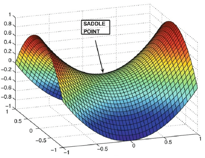
Saddle points
A saddle point represents a local minimum along some subspace of the loss function surface. The gradient can vanish in these regions, even though the loss may still be high. It is rather difficult to escape in practice.
Cliffs
Cliff edges can spike gradients so large that unreasonably large jumps take place, this kind of extreme is dangerous! This can be solved with gradient clipping where we instead move: \(\boldsymbol{\theta}^{i+1}=\boldsymbol{\theta}^i-max\{\gamma \nabla\mathcal{L},\bar{\gamma}\}\) where \(\bar{\gamma}\) is chosen as the maximal move size.
Practical advice
- Monitor the gradient norm during fitting
- For activation functions, favour ReLU variants over sigmoid when possible. Helps avoid vanishing gradients due to activation
- Use ‘momentum’ in gradient method to combat ill-conditioning
- Use gradient clipping if cliffs seem to be a problem (see monitoring to help choose clipping value)
- Use mini-batch estimation of gradient. Partition training sample observations \(\{1,2,...,n\}\) into disjoint sets: \(\mathcal{I_i}\cap\mathcal{I_i}=\emptyset, \; i\neq j\) and \(\cup_j\mathcal{I_j}=\{1,...,n\}\), and perform many gradient updates per scan (one scan over the whole data is often called one Epoch) over data.
Advanced Gradient Descent Algorithms
We now explore a number of advanced Gradient Descent Algorithms that you are very likely to use in practice (the “optimizer” you need to specify when you build neural networks).
Stochastic gradient descent (SGD)
Partition training sample observations \(\{1,...,n\}\) into disjoints sets \(\mathcal{I_1},...,\mathcal{I_m}\) Start \(k=0\). While a stopping criterion not met: - for \(j=1,...,m\) - \(k\leftarrow k+1\) - \(\hat{\boldsymbol{g}}=\frac{1}{|\mathcal{I}|}\nabla\sum _{i\in \mathcal{I}}\mathcal{L}(\hat{p}(\boldsymbol{x}_i),\boldsymbol{y}_i;\boldsymbol{\theta})\) - \(\boldsymbol{\theta}\leftarrow \boldsymbol{\theta}-\epsilon_k \hat{\boldsymbol{g}}\) - if stopping criterion met, break - Resample a new partition (batch), continue
This algorithm in theory requires \(\sum_{k=1}^{\infty}\epsilon_k=\infty\) and \(\sum_{k=1}^{\infty}\epsilon_k^2<\infty\) for convergence. However, we commonly choose linear decay until a threshold.
SGD + (Nesterov) momentum
Momentum accumulates exponentially decaying average to reduce poor movement from noisy (mini-batch) or ill-conditioned updates.
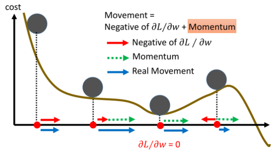
A classic deterministic version is given by: \[\boldsymbol{v}\leftarrow\alpha\boldsymbol{v}-\frac{\epsilon}{|\mathcal{I}|}\nabla\sum _{i\in \mathcal{I}}\mathcal{L}(\hat{p}(\boldsymbol{x}_i),\boldsymbol{y}_i;\boldsymbol{\theta})\] \[\boldsymbol{\theta}\leftarrow\boldsymbol{\theta}+\boldsymbol{v}\]
Or, stochastic version of famous Nesterov momentum method (\(O(k^{-2})\) in convex case): \[\boldsymbol{v}\leftarrow\alpha\boldsymbol{v}-\frac{\epsilon}{|\mathcal{I}|}\nabla\sum _{i\in \mathcal{I}}\mathcal{L}(\hat{p}(\boldsymbol{x}_i),\boldsymbol{y}_i;\boldsymbol{\theta}+\alpha\boldsymbol{v})\] \[\boldsymbol{\theta}\leftarrow\boldsymbol{\theta}+\boldsymbol{v}\] Commonly \(\alpha=0.5, 0.9, 0.99\) and adapted over time (another tuning parameter for optimization).
RMSProp
Root Mean Squared Propagation, or RMSProp, is an extension of gradient descent and the adaptive gradient that seeks (i) automatically adaptive method so schedules of parameters not needed; and (ii) to learn at different rates in different directions. \[\boldsymbol{g}\leftarrow\frac{1}{|\mathcal{I}|}\nabla\sum _{i\in \mathcal{I}}\mathcal{L}(\hat{p}(\boldsymbol{x}_i),\boldsymbol{y}_i;\boldsymbol{\theta})\] \[\boldsymbol{r}\leftarrow \rho \boldsymbol{r}+(1-\rho)\boldsymbol{g}\odot\boldsymbol{g}\] \[\boldsymbol{\theta}\leftarrow \boldsymbol{\theta}-\frac{\epsilon}{\sqrt{\delta+\boldsymbol{r}}}\odot\boldsymbol{g}\] typically \(\delta\approx 10^{-6}\), \(\epsilon\) and \(\rho\) are tuning parameters.
From RMSProp, we can also add Nesterov acceleration to this scheme. And Adaptive Moment Estimation (Adam) is simply a combination of Momentum and RMSprop.
General comments
- And there are many more. Adam is a reasonable default to use.
- Sadly no theoretical guidance on one optimisation scheme being uniformly superior to another.
- Second order methods (Newton etc) unlikely to provide a solution soon due to substantially greater compute cost.
- General theme is that there are limits to what optimisation can achieve … make models which are easier to optimise rather than waiting for a better optimiser! (ie more linear functions enabling good gradient flows, less sigmoids unless necessary)
3.5 Overfitting
The appeal of deep learning’s ability to fit arbitrarily complex functional relationships is also a potential Achilles’ heel — we’ve seen how easily even less flexible classical ML methods can overfit. We now have a lightning review of strategies to combat overfitting.
L1/L2 regularisation
We have seen L1 (aka Lasso) and L2 (aka Ridge) regularisation in regression. We can embed these techniques into our loss function to regularise all the many stacked linear models, for example using ridge: \[\tilde{\mathcal{L}}(\hat{p}(\boldsymbol{x}_i),\boldsymbol{y}_i;\boldsymbol{\theta})=\mathcal{L}(\hat{p}(\boldsymbol{x}_i),\boldsymbol{y}_i;\boldsymbol{\theta})+\lambda\sum_l\sum_j ||\boldsymbol{w}_j^{[l]}||_2^2\] where \(\lambda\) is another tunning parameter for optimization.
Data augmentation
The more data we have the better our algorithm will generalise, but we only have finite data … so generate fake data!
- In image classification, probably want deep net to be invariant to rotation, scaling and translation… so apply these operations and add to the training data!
- For regular data, apply tiny noise to input data can be shown to be equivalent to regularising the weights.
- For speech recognition, want the deep net to be invariant to certain sound distortions or background noise.
- …
Obviously this is quite an application specific approach, but can help with generalisability of a deep net greatly just by making more data from the data you already have.
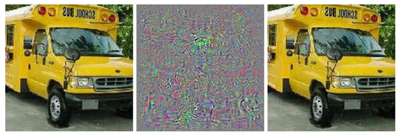
Adversarial training
Similar to data augmentation, but post model fit. Run an optimiser on existing data looking for minimal perturbation that changes classification. The Figure below shows an example that after applying the perturbation (Middle panel) to the original image (Left panel) which the fitted model correctly classifies it as school bus, the newly fitted model will classify the perturbed image (Right panel) to ostrich. Adding this new perturbed image to the training data would help to train the model better.
Bagging
Our old friend bagging lives on in the deep learning world. In fact, remember, a deep neural network is essentially a stochastic model! Every time you fit even with same parameters and same data, the final fit is slightly different due to SGD. This can be enough to induce sufficiently uncorrelated errors to make averaging deep nets refitted on full training data useful. Otherwise, actually do bootstrap and/or fits with slightly different parameterisations.
Dropout
Dropout is a remarkably effective and powerful technique. Random eliminate some inputs and hidden neurons from training (don’t include in forward or backward passes). Change what is “dropped out” each time you draw a new mini-batch in training. To a first-order approximation, this is like bagging many many neural networks: any network that is a subnetwork of the design chosen! Unlike bagging, dropout actually reduces the computational cost but we get the improvement in generalisation. Input layer dropout \(0-0.2\) and hidden layer dropout \(0-0.5\) is common.
3.6 Convolutional neural networks (CNNs)
Convolutional neural networks are especially suited to image data, though not exclusively. They were directly inspired by the Nobel prize winning work of Hubel & Wiesel, neuroscientists who measured individual neuronal activity in a cat’s visual cortex! CNNs require far fewer parameters to do effective image recognition than an equivalent multi-layer perceptron layout requires, but it’s all built out of the same foundations.
Convolution shifts a small kernel over the input tensor (see the Figure below), producing the equivalent of flattened inner product. Kernel contains the parameters, often 2x2, 3x3, or similarly small even for large images.
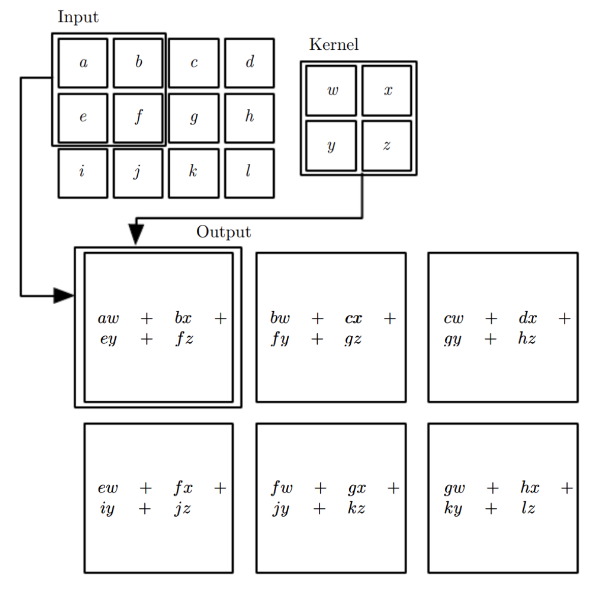
There exists a matrix representation of this operation, i.e. a Toeplitz matrix applied to the flattened input is equivalent.
Although CNNs lead to a much more sparsely connected hidden layer, e.g. each input pixel only influences the restricted number of neurons, this structure (as indicated by the Toeplitz matrix) results in extensive parameter sharing and reduces the dimensionality of the neural network for faster computation and easier fitting.
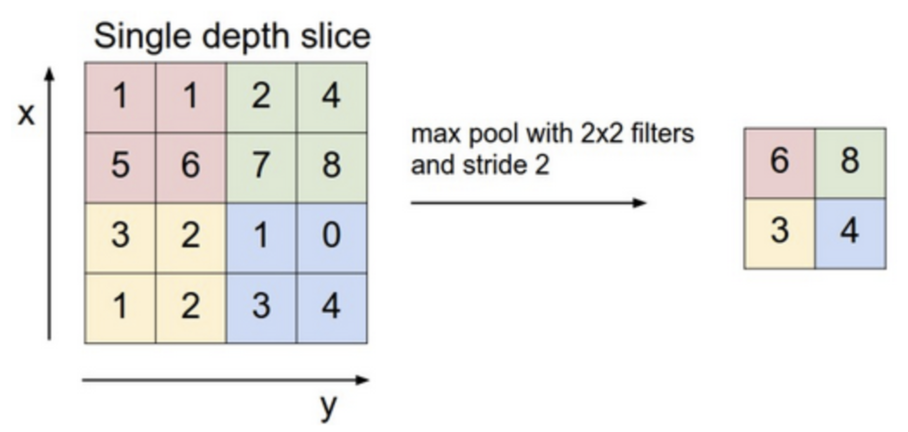
In CNNs, pooling layers are often used to provide an approach to down sampling feature maps by summarizing the presence of features in patches of the feature map. Two common pooling methods are average pooling and max pooling (see an example of max pooling in the Figure below) that summarize the average presence of a feature and the most activated presence of a feature respectively.
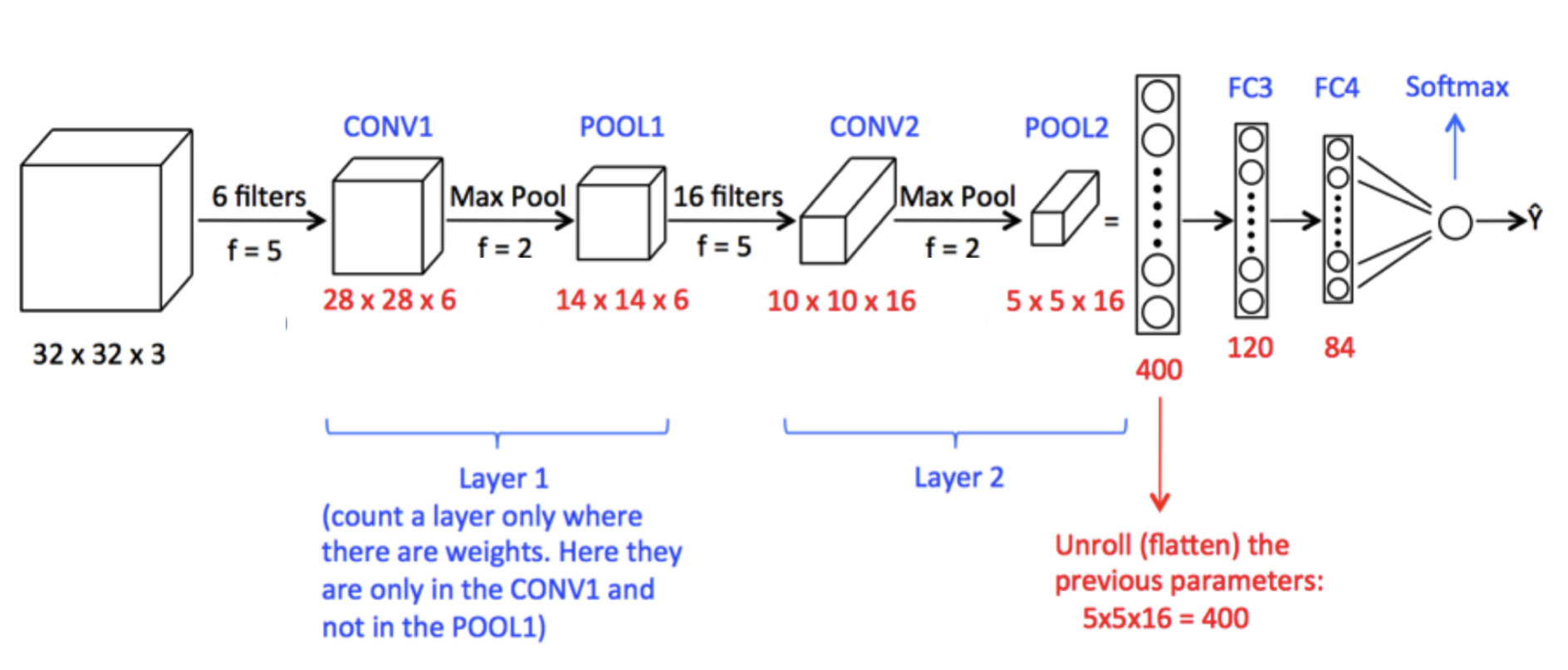
The following Figure provides a classic example of CNNs, the input layer is a three dimensional tensor which represents a colored image. Six 5x5 convolutional kernels (filters) are applied to the input layer and then max pooled to a 14x14x6 first hidden layer, then the first layer is fed into the second convolutional layer before being flattened and fed forward through two more fully connected layers and eventually using softmax activation function to produce a probabilistic forecast.
3.7 Autoencoder
Autoencoders are an unsupervised learning technique in which we leverage neural networks for the task of feature learning. An autoencoder is a neural network whose job it is to take input \(\boldsymbol{x}\) and predict \(\boldsymbol{x}\). Simply put, we need to add a bottleneck layer whose dimension is much smaller than the input.
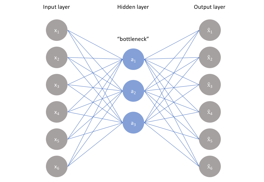
This network can be trained by minimizing the reconstruction error, \(\mathcal{L}(\boldsymbol{x},\hat{\boldsymbol{x}})\), which measures the differences between our original input and the consequent reconstruction.
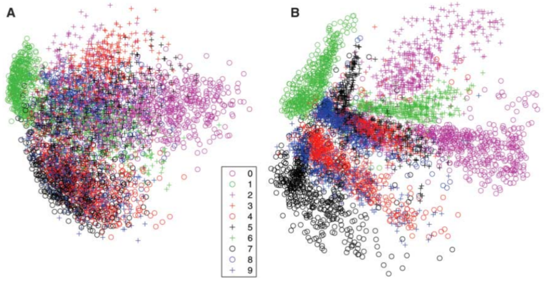
Because neural networks are capable of learning nonlinear relationships, this can be thought of as a more powerful (nonlinear) generalization of PCA. Whereas PCA attempts to discover a lower dimensional hyperplane which describes the original data, autoencoders are capable of learning nonlinear manifolds (a manifold is defined in simple terms as a continuous, non-intersecting surface). The following Figure shows a comparison between PCA (Panel A) and Autoencoder (Panel B) when they are applied to mnist handwritten digits Data and compress the original data into 2 dimensions only.