Chapter 5 Model and hypothesis testing
5.1 Fitting the Generalized Linear Model for Each Gene
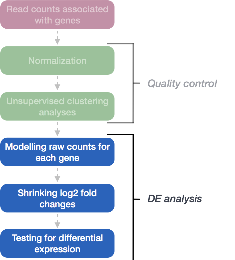
The final step in the DESeq2 workflow involves fitting a Negative Binomial (NB) model to each gene’s expression data and performing differential expression testing.
 Modeling RNA-Seq Counts
DESeq2 uses a negative binomial generalized linear model (GLM) to model the RNA-Seq counts for each gene. A GLM is a flexible statistical framework similar to linear regression, but it can handle data that doesn’t follow a normal distribution, such as count data.
Modeling RNA-Seq Counts
DESeq2 uses a negative binomial generalized linear model (GLM) to model the RNA-Seq counts for each gene. A GLM is a flexible statistical framework similar to linear regression, but it can handle data that doesn’t follow a normal distribution, such as count data.
For DESeq2, two key components are needed to fit the NB model: the size factor (which normalizes for differences in sequencing depth) and the dispersion estimate (which accounts for biological variability between samples). Additionally, the model uses a design matrix that incorporates the experimental conditions and covariates of interest. By fitting the NB model, DESeq2 estimates the mean counts and dispersion for each gene and uses statistical tests, such as the Wald test, to evaluate whether the observed differences between conditions are statistically significant.
The general form of the negative binomial model is shown below:
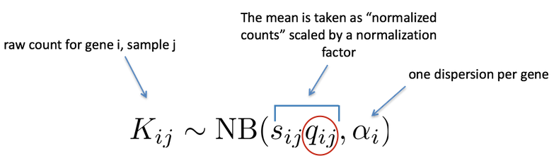
Where:
\(K_{ij}\) are the raw counts for gene \(i\) in sample \(j\)
\(q_{ij}\) represents the true expression level of for gene \(i\) in sample \(j\)
\(sizeFactor_{j}\) is the sizeFactor for sample \(j\)
\(\alpha_{i}\) is the dispersion parameter for gene \(i\)
Estimating Coefficients Using Maximum Likelihood After estimating the dispersion parameter (\(\alpha_{i}\)) for each gene, DESeq2 fits the model again to estimate the regression coefficients (\(\beta\)) while keeping \(\alpha_{i}\) fixed. These coefficients (\(\beta\)) are determined for each sample group using maximum likelihood estimation (MLE), which maximizes the log-likelihood of the Negative Binomial distribution. The \(\beta\) values describe the relationship between the mean expression (\(\mu_{i}\)) and the experimental conditions (e.g., treated vs. control).
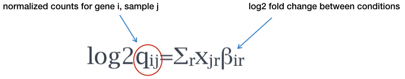
The mean expression (\(\mu_{i}\)) is modeled as a function of the covariates in the design matrix (\(X_{i}\)) and the regression coefficients (\(\beta\)):
\[log(\mu_{ij}) = X_{ij} \beta\]
or equivalently:
\[\mu_{ij} = exp{X_{ij} \beta}\]
Where:
\(\mu_{ij}\) is the expected count for gene \(i\) in sample \(j\)
\(X_{ij}\) represents the covariates (design matrix) for gene \(i\) and sample \(j\)
\(\beta\) is the vector of coefficients (log2 fold changes) for the covariates
The log-likelihood for the regression coefficients \(\beta\) is maximized by substituting the mean (\(\mu_{ij}\)) with \(exp{X_{ij} \beta}\) into the negative binomial likelihood function.
Log2 Fold Change and Adjustments The estimated \(\beta\) coefficients represent the log2 fold changes between different sample groups. However, log2 fold changes are noisier when gene counts are low due to the higher dispersion seen in low-count genes. To address this, the log2 fold changes calculated by the model are adjusted to improve reliability.
 In the case of our dataset, the design has three levels, and the model can be written as:
\[ y = \beta_0 + \beta_1 x_{mov10kd} + \beta_2 x_{mov10oe} \]
Where:
\(y\) is the log2 of the fitted counts for each gene
\(\beta_0\) is the log2 average of the reference group (e.g. “control”)
\(\beta_1\) is the log2 fold change between “Mov10_kd” and the reference group “control”
\(\beta_2\) is the log2 fold change between “Mov10_oe” and the reference group “control”
\(x_{mov10kd}\) and \(x_{mov10oe}\) are indicators of whether a sample belongs to the “Mov10_kd” or “Mov10_oe” groups, respectively.
The \(\beta\) coefficients are the estimates for the log2 fold changes for each sample group. However, log2 fold changes are inherently noisier when counts are low due to the large dispersion we observe with low read counts. To avoid this, the log2 fold changes calculated by the model need to be adjusted.
5.2 Shrunken Log2 Fold Changes (LFC)
Why Are Shrunken Log2 Fold Changes Used in DESeq2?
In RNA-Seq analysis, genes with low counts or high variability often produce large or erratic log2 fold change (logFC) estimates, even when the actual difference between conditions is small. These highly variable estimates can skew downstream analysis. To address this, DESeq2 applies Empirical Bayes shrinkage to bring extreme log2 fold changes closer to more reasonable values.
Handling Noisy Estimates:
Genes with low counts or high dispersion values tend to have noisier log2 fold changes. Shrinking these estimates toward moderate values improves accuracy and reduces variability.
Reducing the Influence of Outliers:
By shrinking extreme log2 fold changes, DESeq2 reduces the impact of outlier genes, that may extreme counts due to technical artifacts or random variation. DESeq2 applies shrinkage particularly when the information for a gene is low, such as:
- Low counts
- High dispersion values
How Does Shrinkage Work for Log2 Fold Changes? Similar to how dispersion shrinkage works, log2 fold change estimates are stabilized using information from all genes. A normal distribution is fitted to the LFC estimates across genes, which serves as a prior. This prior is then used to shrink the estimates for genes with high uncertainty or variability, pulling noisy LFC estimates closer to the global average. Genes with low counts or a small number of replicates undergo more shrinkage, while genes with higher counts and reliable data undergo less shrinkage.
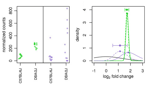
Illustration taken from the DESeq2 paper.
In the figure above, both the green and purple genes have the same mean values across two sample groups (C57BL/6J and DBA/2J), but the green gene shows little variation while the purple gene has high variation. The shrunken log2 fold change for the green gene (dotted line) is nearly the same as its unshrunken estimate (vertex of the green solid line). However, the LFC estimates for the purple gene is pulled much closer to the prior distribution (black line) due to its higher dispersion.
Generating Shrunken LFC Estimates
To generate shrunken log2 fold change estimates, you can run the lfcShrink() function on your results object:
5.3 Statistical test for LFC estimates: Wald test
DESeq2 uses the Wald test as the default method for hypothesis testing when comparing two groups. This test evaluates the significance of the log2 fold change (LFC) for each gene by comparing the LFC estimate to its standard error.
The Wald test proceeds as follows:
The log2 fold change is divided by its standard error, yielding a z-statistic (how many standard deviations an estimate (in this case, the LFC) is away from its expected value under the null hypothesis).
The z-statistic is compared to a standard normal distribution to compute a p-value.
If the p-value is small enough, the null hypothesis (LFC = 0) is rejected, indicating evidence of differential expression.
DESeq2 Workflow Overview:
In DESeq2, the Wald test is an integral part of the hypothesis testing procedure. The overall workflow follows these steps:
- Estimate Size Factors
- Estimate Dispersions
- Fit the Negative Binomial GLM
- Perform Hypothesis Testing (using the Wald test for LFC estimates)
Creating Contrasts for Hypothesis Testing
In DESeq2, contrasts define the specific groups to compare for differential expression testing. There are two ways to create contrasts:
Default Comparison:
DESeq2 automatically uses the base level of the factor of interest, determined alphabetically, as the baseline for comparisons (reference).
Manual Specification:
You can manually specify the contrast using the contrast argument in the results() function. The last group in the contrast becomes the base for comparison (reference).
# DO NOT RUN!
contrast <- c("condition", "level_to_compare", "base_level")
results(dds, contrast = contrast, alpha = alpha_threshold)
The alpha parameter in DESeq2 sets the significance cutoff used for optimizing independent filtering. The alpha value is used to determine the criteria for independent filtering, meaning DESeq2 will try to optimize the filtering process to maximize the number of genes with adjusted p-values below the alpha threshold.
The filtering step removes genes that are unlikely to achieve an adjusted p-value (FDR) below this alpha value (i.e., those with low counts or low statistical power). However, the primary criterion used for independent filtering is the mean normalized count of the genes.
By default, alpha is set to 0.1, meaning that genes with an adjusted p-value (false discovery rate, or FDR) below this threshold will be considered significant. However, you can adjust the alpha parameter to reflect a more stringent FDR threshold, such as 0.05, depending on your analysis needs.
5.3.1 MOV10 DE Analysis: Contrasts and Wald Tests
In our MOV10 dataset, there are three groups, allowing for the following pairwise comparisons:
- Control vs. Mov10 overexpression
- Control vs. Mov10 knockdown
- Mov10 knockdown vs. Mov10 overexpression
For this analysis, we are primarily interested in comparisons #1 and #2. The design formula we provided earlier (~ sampletype) defines our main factor of interest.
Building the Results Table
To build the results table, we use the results() function. You can specify the contrast to be tested using the contrast argument. In this example, we’ll save the unshrunken and shrunken results of Control vs. Mov10 overexpression to different variables. We’ll also set the alpha to 0.05, which is the significance cutoff for independent filtering.
## Define contrasts, extract results table, and shrink log2 fold changes
contrast_oe <- c("sampletype", "MOV10_overexpression", "control")

res_tableOE_unshrunken <- results(dds, contrast = contrast_oe, alpha = 0.05)

resultsNames(dds)
## [1] "Intercept"
## [2] "sampletype_MOV10_knockdown_vs_control"
## [3] "sampletype_MOV10_overexpression_vs_control"res_tableOE <- lfcShrink(dds = dds, coef = "sampletype_MOV10_overexpression_vs_control",
res = res_tableOE_unshrunken)## using 'apeglm' for LFC shrinkage. If used in published research, please cite:
## Zhu, A., Ibrahim, J.G., Love, M.I. (2018) Heavy-tailed prior distributions for
## sequence count data: removing the noise and preserving large differences.
## Bioinformatics. https://doi.org/10.1093/bioinformatics/bty895The Importance of Contrast Order in Log2 Fold Change (LFC) Calculations
In DESeq2, when you specify a contrast, you are defining a comparison between two levels of a factor (in this case, the “sampletype” factor). The order of the names in the contrast determines the direction of the fold change reported. The first group listed in the contrast (“MOV10_overexpression”) is the group you are comparing. The second group listed in the contrast (“control”) is the baseline or reference group, against which the comparison is made. A positive log2 fold change means that gene expression is higher in the “MOV10_overexpression” group compared to “control”. A negative log2 fold change means that gene expression is lower in the “MOV10_overexpression” group compared to “control”.
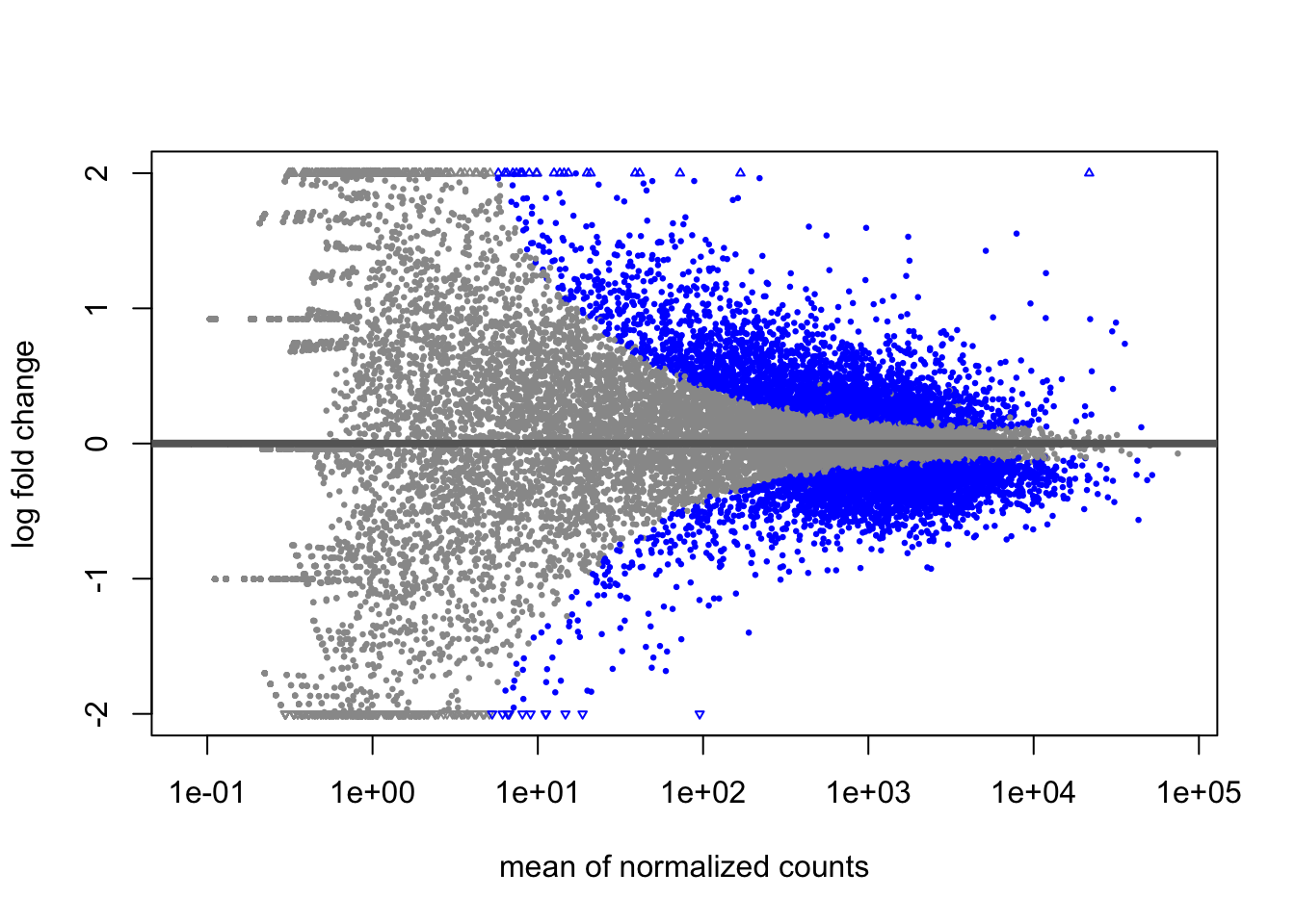
MA Plot
An MA plot is a useful visualization for exploring differential expression results. It shows the relationship between the mean of the normalized counts (on the x-axis) and the log2 fold changes (on the y-axis) for all genes tested. Genes that are significantly differentially expressed are highlighted in color for easier identification.
This plot is also a great way to illustrate the effect of LFC shrinkage. DESeq2 provides a simple function to generate an MA plot.
Unshrunken Results:
Shrunken results:
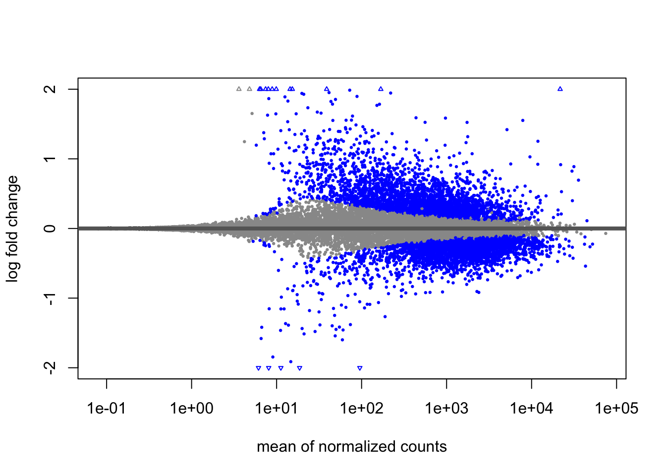
In addition to comparing LFC shrinkage, the MA plot helps you evaluate the magnitude of fold changes and how they are distributed relative to mean expression. You would expect to see significant genes across the full range of expression levels.
MOV10 DE Analysis: Exploring the Results
The results table in DESeq2 looks similar to a data.frame and can be treated like one for accessing or subsetting data. However, it is stored as a DESeqResults object, which is important to keep in mind when working with visualization tools.
## [1] "DESeqResults"
## attr(,"package")
## [1] "DESeq2"
Let’s go through some of the columns in the results table to get a better idea of what we are looking at. To extract information regarding the meaning of each column we can use mcols():
## DataFrame with 5 rows and 2 columns
##                        type            description
##                 <character>            <character>
## baseMean       intermediate mean of normalized c..
## log2FoldChange      results log2 fold change (MA..
## lfcSE               results posterior SD: sample..
## pvalue              results Wald test p-value: s..
## padj results BH adjusted p-valuesbaseMean: mean of normalized counts for all sampleslog2FoldChange: log2 fold change estimatelfcSE: standard error of the LFC estimatestat: Wald statisticpvalue: P-value from the Wald testpadj: Adjusted p-values using the Benjamini-Hochberg method
Now let’s take a look at what information is stored in the results:
## log2 fold change (MAP): sampletype MOV10_overexpression vs control
## Wald test p-value: sampletype MOV10 overexpression vs control
## DataFrame with 6 rows and 5 columns
##               baseMean log2FoldChange     lfcSE    pvalue      padj
##              <numeric>      <numeric> <numeric> <numeric> <numeric>
## 1/2-SBSRNA4  45.652040     0.16820235  0.209100 0.1610752 0.2655661
## A1BG         61.093102     0.13645896  0.176779 0.2401909 0.3603094
## A1BG-AS1    175.665807    -0.04046122  0.116928 0.6789312 0.7748342
## A1CF          0.237692     0.00626747  0.210057 0.7945932        NA
## A2LD1        89.617985     0.29017719  0.195395 0.0333343 0.0741149
## A2M           5.860084    -0.09619722  0.233561 0.1057823 0.1900466
Interpreting p-values Set to NA
In some cases, p-values or adjusted p-values may be set to NA for a gene. This happens in three scenarios:
Zero counts: If all samples have zero counts for a gene, its baseMean will be zero, and the log2 fold change, p-value, and adjusted p-value will all be set to NA.
Outliers: If a gene has an extreme count outlier, its p-values will be set to NA. These outliers are detected using Cook’s distance.
Low counts: If a gene is filtered out by independent filtering for having a low mean normalized count, only the adjusted p-value will be set to NA.
Multiple Testing Correction
In the results table, we see both p-values and adjusted p-values. Which should we use to identify significantly differentially expressed genes?
If we used the p-value directly from the Wald test with a significance cut-off of p < 0.05, that means there is a 5% chance it is a false positives. Each p-value is the result of a single test (single gene). The more genes we test, the more we inflate the false positive rate. This is the known as the multiple testing problem. For example, testing 20,000 genes with a p-value threshold of 0.05 would result in 1,000 genes being significant by chance alone. If we found 3000 genes to be differentially expressed total, 150 of our genes are false positives. We would not want to sift through our “significant” genes to identify which ones are true positives.
DESeq2 helps reduce the number of genes tested by removing those genes unlikely to be significantly DE prior to testing, such as those with low number of counts and outlier samples (gene-level QC). However, we still need to correct for multiple testing to reduce the number of false positives, and there are a few common approaches: To address this, we apply multiple testing correction.
DESeq2 corrects p-values using the Benjamini-Hochberg (BH) method by default, which controls the false discovery rate (FDR). Other methods, like Bonferroni, are available but tend to be more conservative and lead to higher rates of false negatives.
In most cases, we should use the adjusted p-values (BH-corrected) to identify significant genes.
5.3.2 MOV10 DE Analysis: Control vs. Knockdown
After examining the overexpression results, let’s move on to the comparison between Control vs. Knockdown. We’ll use contrasts in the results() function to extract the results table and store it in the res_tableKD variable.
## Define contrasts, extract results table, and shrink log2 fold changes
contrast_kd <- c("sampletype", "MOV10_knockdown", "control")

res_tableKD_unshrunken <- results(dds, contrast = contrast_kd, alpha = 0.05)

resultsNames(dds)
## [1] "Intercept"
## [2] "sampletype_MOV10_knockdown_vs_control"
## [3] "sampletype_MOV10_overexpression_vs_control"# We can also specify contrasts using `coef` argument in `lfcShrink()`
res_tableKD <- lfcShrink(dds, coef = 2, res = res_tableKD_unshrunken)## using 'apeglm' for LFC shrinkage. If used in published research, please cite:
## Zhu, A., Ibrahim, J.G., Love, M.I. (2018) Heavy-tailed prior distributions for
## sequence count data: removing the noise and preserving large differences.
## Bioinformatics. https://doi.org/10.1093/bioinformatics/bty8955.4 Summarizing Results
To summarize the results, DESeq2 offers the summary() function, which conveniently reports the number of genes that are significantly differentially expressed at a specified threshold (default FDR < 0.05). Note that, even though the output refers to p-values, it actually summarizes the results using adjusted p-values (padj/FDR).
Let’s start by summarizing the results for the OE vs. control comparison:
##
## out of 19748 with nonzero total read count
## adjusted p-value < 0.05
## LFC > 0 (up)       : 3103, 16%
## LFC < 0 (down)     : 3408, 17%
## outliers [1]       : 0, 0%
## low counts [2]     : 4171, 21%
## (mean count < 5)
## [1] see 'cooksCutoff' argument of ?results
## [2] see 'independentFiltering' argument of ?results
In addition to reporting the number of up- and down-regulated genes at the default significance threshold, this function also provides information on:
- Number of genes tested (genes with non-zero total read count)
- Number of genes excluded from multiple test correction due to low mean counts
5.4.1 Extracting Significant Differentially Expressed Genes
In some cases, using only the FDR threshold doesn’t sufficiently reduce the number of significant genes, making it difficult to extract biologically meaningful results. To increase stringency, we can apply an additional fold change threshold.
Although the summary() function doesn’t include an argument for fold change thresholds, we can define our own criteria.
Let’s start by setting the thresholds for both adjusted p-value (FDR < 0.05) and log2 fold change (|log2FC| > 0.58, corresponding to a 1.5-fold change):
Next, we’ll convert the results table to a tibble for easier subsetting:
Now, we can filter the table to retain only the genes that meet the significance and fold change criteria:
sigOE <- res_tableOE_tb %>%
    filter(padj < padj.cutoff & abs(log2FoldChange) > lfc.cutoff)

# Save the results for future use
saveRDS(sigOE, "data/sigOE.RDS")
Exercise points = +3
How many genes are differentially expressed in the Overexpression vs. Control comparison based on the criteria we just defined? Does this reduce the number of significant genes compared to using only the FDR threshold?
Click here to see the solution
nrow(sigOE)Does this reduce our results?
Click here to see the solution
nrow(sigOE)

            nrow(res_tableOE)

            100 - (nrow(sigOE)/nrow(res_tableOE) *100)

            "Yes, it is decreased from 23368 to 951
            (representing about 4% of the genes)."
5.4.2 MOV10 Knockdown Analysis: Control vs. Knockdown
Next, let’s perform the same analysis for the Knockdown vs. Control comparison. We’ll use the same thresholds for adjusted p-value (FDR < 0.05) and log2 fold change (|log2FC| > 0.58).
res_tableKD_tb <- res_tableKD %>%
    data.frame() %>%
    rownames_to_column(var = "gene") %>%
    as_tibble()

sigKD <- res_tableKD_tb %>%
    dplyr::filter(padj < padj.cutoff & abs(log2FoldChange) > lfc.cutoff)

# We'll save this object for use in the homework
saveRDS(sigKD, "data/sigKD.RDS")
How many genes are differentially expressed in the Knockdown compared to Control?
Click here to see the solution
nrow(sigKD)Now that we have subsetted our data, we are ready for visualization!