Chapter 1 Differential gene expression (DGE) analysis overview

The goal of RNA-seq is to perform differential expression testing to determine which genes are expressed at different levels between conditions. These genes can offer biological insight into the processes affected by the condition(s) of interest.

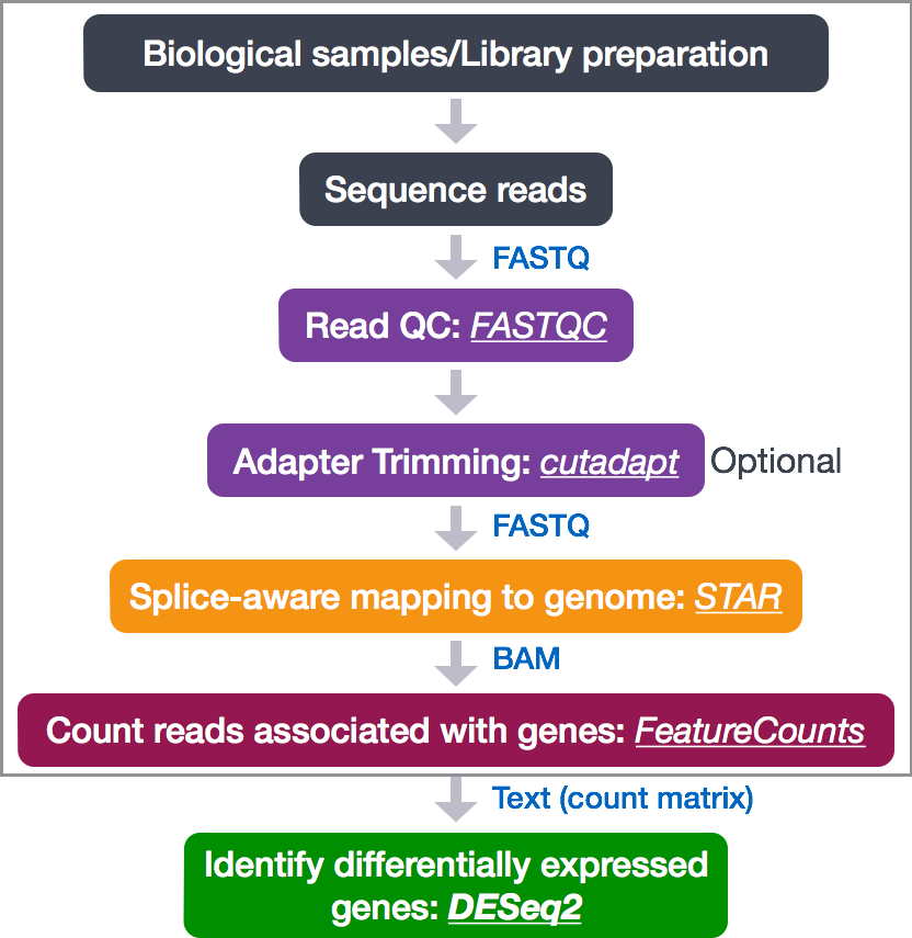
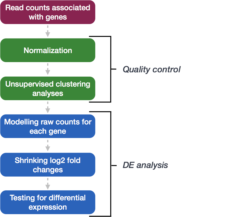
To determine the expression levels of genes, our RNA-seq workflow follows the steps detailed in the image below inside the box. All steps are performed on the command line (Linux/Unix) through the generation of read counts per gene as discussed in Corey’s lectures. The differential expression analysis and any downstream functional analysis are generally performed in R using R packages specifically designed for the complex statistical analyses required to determine whether genes are differentially expressed starting from the count matrices.

In the next few lessons, we will walk you through an end-to-end gene-level RNA-seq differential expression workflow using various R packages. We will start with the count matrix, perform exploratory data analysis for quality assessment and to explore the relationship between samples, perform differential expression analysis, and visually explore the results prior to performing downstream functional analysis.

1.1 Review of the dataset

We will be using the full count matrix from the RNA-seq dataset that is part of a larger study described in Kenny PJ et al, Cell Rep 2014 investigating the interactions between genes potentially involved in Fragile X syndrome (FXS). FXS is a genetic disorder and the leading cause of inherited intellectual disabilities like autism. FXS is caused by aberrant production of a protein called Fragile X Messenger Ribonucleoprotein (FMRP) that is needed for brain development. People who have FXS do not make this protein. The authors demonstrated that FMRP associates with another RNA-binding protein MOV10 (Mov10 RISC Complex RNA Helicase) and acts to regulate the translation of a subset of RNAs.

What is the function of FMRP and MOV10?

FMRP is “most commonly found in the brain, is essential for normal cognitive development and female reproductive function. Mutations of this gene can lead to fragile X syndrome, mental retardation, premature ovarian failure, autism, Parkinson’s disease, developmental delays and other cognitive deficits.” - from wikipedia

MOV10 is a putative RNA helicase that is associated with FMRP in the context of the microRNA pathway. MOV10 has a role in regulating translation: it facilitates microRNA-mediated translation of some RNAs, but it also increases expression of other RNAs.

The aim of the RNAseq part of the study was to characterize the transcription expression patterns of FMRP and MOV10 to identify overlapping target genes which would suggest that these genes are regulated by the MOV10-FMRP complex.

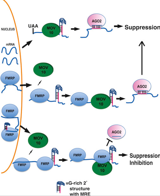
Model for MOV10-FMRP** Association in Translation Regulation. Top: fate of RNAs bound by MOV10. MOV10** binds the 3′ UTR-encoded G-rich structure to reveal MREs for subsequent AGO2 association. Middle: fate of RNAs bound by FMRP. FMRP binds RNAs in the nucleus. Upon export, FMRP recruits MOV10, which ultimately unwinds MREs for association with AGO2. Bottom: FMRP recruits MOV10 to RNAs; however, binding of both FMRP and MOV10 in proximity of MRE blocks association with AGO2. Red line indicates MRE.

RNA-seq was performed on HEK293F cells that were either transfected with a MOV10 transgene, or siRNA to knock down Mov10 expression, or non-specific (irrelevant) siRNA. This resulted in 3 conditions Mov10 oe (over expression), Mov10 kd (knock down) and Irrelevant kd, respectively. The number of replicates is as shown below.

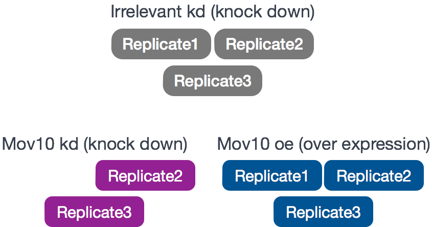
Using these data, we will evaluate transcriptional patterns associated with perturbation of MOV10 expression. Please note that the irrelevant siRNA will be treated as our control condition.

Links to raw data [GEO]: https://www.ncbi.nlm.nih.gov/geo/query/acc.cgi?acc=GSE51443 “Gene Expression Omnibus” [SRA]: https://trace.ncbi.nlm.nih.gov/Traces/sra/?study=SRP031507 “Sequence Read Archive”

Our questions: * What patterns of expression can we identify with the loss or gain of MOV10? * Are there any genes shared between the two conditions?

1.2 Setting up

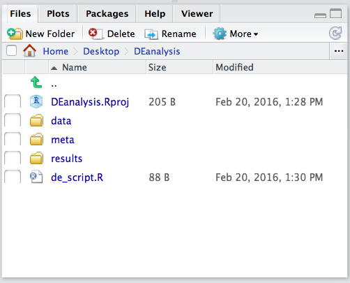
Go to the File menu and open 09-DGE_codebook.Rmd. This should open up a script editor in the top left hand corner. This is where we will be running all commands required for this analysis. Your working directory should have these folders: data, meta and results:

1.2.1 Loading libraries

For this analysis we will be using several R packages, some which have been installed from CRAN and others from Bioconductor. To use these packages (and the functions contained within them), we need to load the libraries. Add the following to your script and don’t forget to comment liberally!

## Setup Bioconductor and CRAN libraries used
library(tidyverse)
library(RColorBrewer)
library(DESeq2)
library(pheatmap)

1.2.2 Loading data

To load the data into our current environment, we will be using the read.table function. We need to provide the path to each file and also specify arguments to let R know that we have a header (header = T) and the first column is our row names (row.names =1). By default the function expects tab-delimited files, which is what we have.

## Load in data
data <- read.table("data/Mov10_full_counts.txt", header = T, row.names = 1)

meta <- read.table("data/Mov10_full_meta.txt", header = T, row.names = 1)

Use class() to inspect our data and make sure we are working with data frames:

### Check classes of the data we just brought in
class(meta)

## [1] "data.frame"

class(data)

## [1] "data.frame"

1.2.3 Viewing data

Make sure your datasets contain the expected samples / information before proceeding to perfom any type of analysis.

head(meta)

	sampletype	MOVexpr
Irrel_kd_1	control	normal
Irrel_kd_2	control	normal
Irrel_kd_3	control	normal
Mov10_kd_2	MOV10_knockdown	low
Mov10_kd_3	MOV10_knockdown	low
Mov10_oe_1	MOV10_overexpression	high

head(data)

	Mov10_kd_2	Mov10_kd_3	Mov10_oe_1	Mov10_oe_2	Mov10_oe_3	Irrel_kd_1	Irrel_kd_2	Irrel_kd_3
1/2-SBSRNA4	57	41	64	55	38	45	31	39
A1BG	71	40	100	81	41	77	58	40
A1BG-AS1	256	177	220	189	107	213	172	126
A1CF	0	1	1	0	0	0	0	0
A2LD1	146	81	138	125	52	91	80	50
A2M	10	9	2	5	2	9	8	4

1.3 Differential gene expression analysis overview

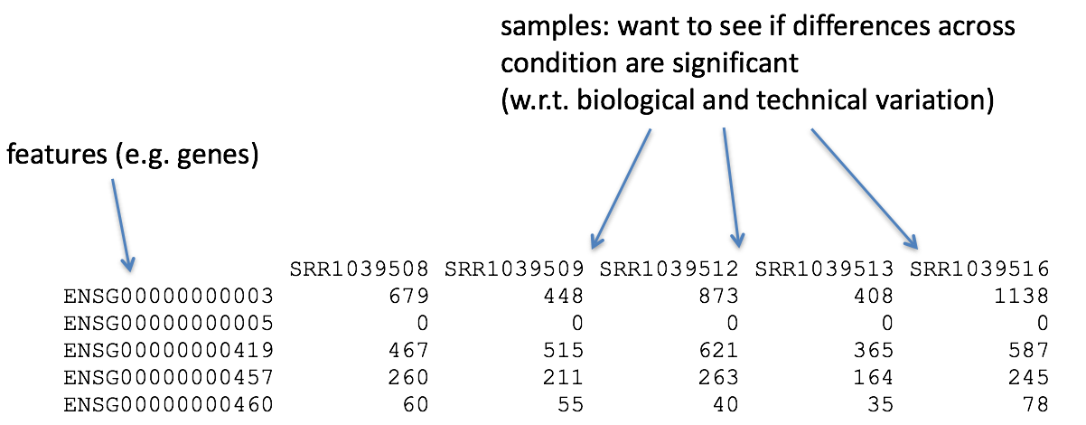
So what does this count data actually represent? The count data used for differential expression analysis represents the number of sequence reads that originated from a particular gene. The higher the number of counts, the more reads associated with that gene, and the assumption that there was a higher level of expression of that gene in the sample.

With differential expression analysis, we are looking for genes that change in expression between two or more groups (defined in the metadata) - case vs. control - correlation of expression with some variable or clinical outcome

Why does it not work to identify differentially expressed gene by ranking the genes by how different they are between the two groups (based on fold change values)?

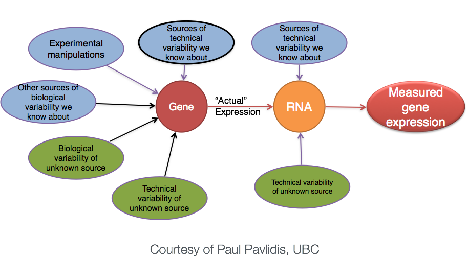
More often than not, there is much more going on with your data than what you are anticipating. Genes that vary in expression level between samples is a consequence of not only the experimental variables of interest but also due to extraneous sources. The goal of differential expression analysis to determine the relative role of these effects, and to separate the “interesting” from the “uninteresting”.

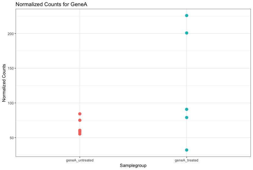
The “uninteresting” presents as sources of variation in your data, and so even though the mean expression levels between sample groups may appear to be quite different, it is possible that the difference is not actually significant. This is illustrated for ‘GeneA’ expression between ‘untreated’ and ‘treated’ groups in the figure below. The mean expression level of geneA for the ‘treated’ group is twice as large as for the ‘untreated’ group, but the variation between replicates indicates that this may not be a significant difference. We need to take into account the variation in the data (and where it might be coming from) when determining whether genes are differentially expressed.

The goal of differential expression analysis is to determine, for each gene, whether the differences in expression (counts) between groups is significant given the amount of variation observed within groups (replicates). To test for significance, we need an appropriate statistical model that accurately performs normalization (to account for differences in sequencing depth, etc.) and variance modeling (to account for few numbers of replicates and large dynamic expression range).

1.3.1 RNA-seq count distribution

To determine the appropriate statistical model, we need information about the distribution of counts. To get an idea about how RNA-seq counts are distributed, let’s plot the counts for a single sample, ‘Mov10_oe_1’:

ggplot(data) + geom_histogram(aes(x = Mov10_oe_1), stat = "bin", bins = 200) + xlab("Raw expression counts") +
    ylab("Number of genes")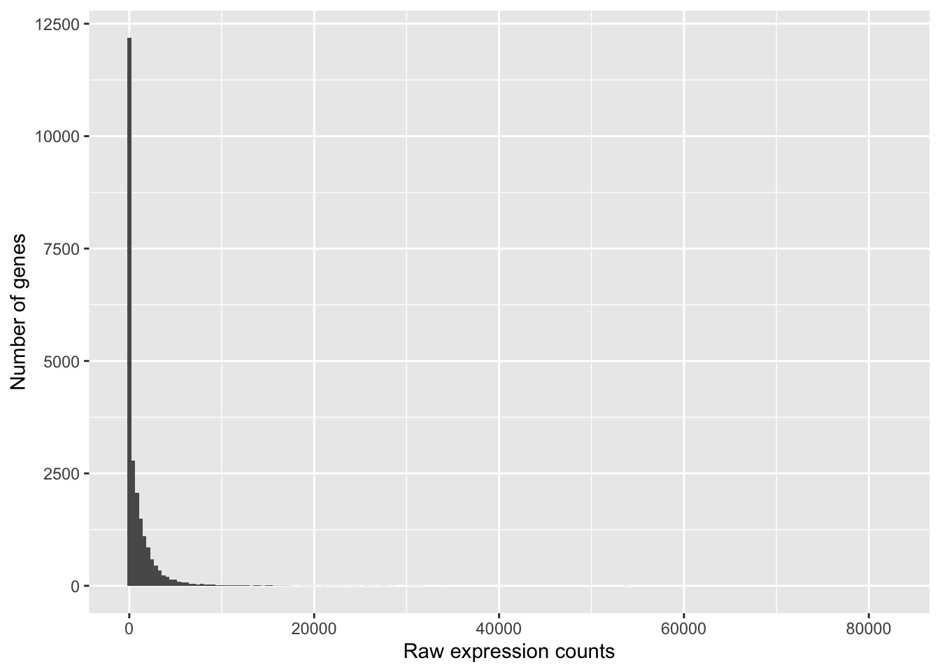

If we zoom in close to zero, we can see a large number of genes with counts of zero:

ggplot(data) + geom_histogram(aes(x = Mov10_oe_1), stat = "bin", bins = 200) + xlim(-5,
    500) + xlab("Raw expression counts") + ylab("Number of genes")

## Warning: Removed 9121 rows containing non-finite outside the scale range
## (`stat_bin()`).

## Warning: Removed 2 rows containing missing values or values outside the scale range
## (`geom_bar()`).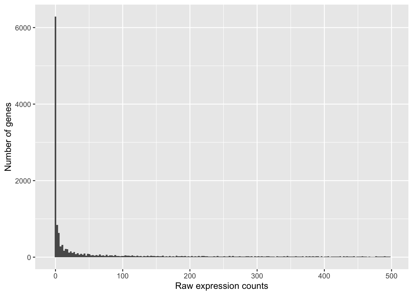

These images illustrate some common features of RNA-seq count data, including a low number of counts associated with a large proportion of genes, and a long right tail due to the lack of any upper limit for expression.

1.3.2 Modeling count data

Count data is often modeled using the binomial distribution. The Binomial distribution is a common probability distribution that models the probability of obtaining one of two outcomes under a given number of parameters. It summarizes the number of trials when each trial has the same chance of attaining one specific outcome. For example, it can give you the probability of getting a number of heads upon tossing a coin a number of times. However, not all count data can be fit with the binomial distribution. The binomial is based on discrete events and used in situations when you have a certain number of cases.

When the number of cases is very large (i.e. people who buy lottery tickets), but the probability of an event is very small (probability of winning), the Poisson distribution is used to model these types of count data.

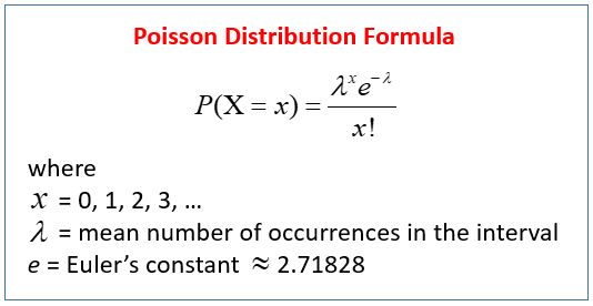
With RNA-seq data, for each sample we have millions of reads being sequenced and the probability of a read mapping to a gene is extremely low. Thus, it would be an appropriate situation to use the Poisson distribution. However, a unique property of this distribution is that the mean == variance given by the single parameter \(\lambda\).

For us to apply a poisson distribution to our data, we first need to find out whether our data fulfills the criteria to use the poisson distribution. To do that we can plot the mean versus variance for the ‘Mov10 overexpression’ replicates:

To calculate the mean and variance of our data, we will use the apply function. The apply function allows you to apply a function to the margins (rows or columns) of a matrix. The syntax for apply is as follows: apply(X, MARGIN, FUN), where X is a matrix, MARGIN is the margin of the matrix to apply the function to (1 = rows, 2 = columns), and FUN is the function to apply.

We will use MARGIN = 1 to apply the mean and variance of the counts for each row (gene) across the ‘Mov10 overexpression’ replicates. We will then create a data frame with the mean and variance of the counts for each gene.

mean_counts <- apply(data[, 3:5], 1, mean)

variance_counts <- apply(data[, 3:5], 1, var)

# for ggplot we need the data to be in a data.frame
df <- data.frame(mean_counts, variance_counts)

Run the following code to plot the mean versus variance for the ‘Mov10 overexpression’ replicates:

ggplot(df) + geom_point(aes(x = mean_counts, y = variance_counts)) + geom_line(aes(x = mean_counts,
    y = mean_counts, color = "red")) + scale_y_log10() + scale_x_log10()

## Warning in scale_y_log10(): log-10 transformation introduced infinite values.

## Warning in scale_x_log10(): log-10 transformation introduced infinite values.

## Warning in scale_y_log10(): log-10 transformation introduced infinite values.

## Warning in scale_x_log10(): log-10 transformation introduced infinite values.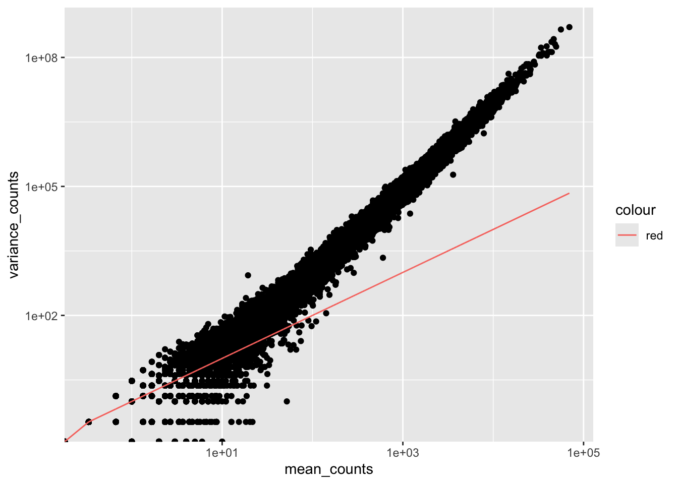

By plotting the mean versus the variance of our data we can easily see that the mean < variance and therefore it does not fit the Poisson distribution. Genes having higher mean counts have even higher variance. Also for gene having low mean counts, there is a scatter of points and we can see that there is variability even in the variance. To account for this extra variance we need a new model.

The model that fits best, given this type of variability between replicates, is the Negative Binomial (NB) model. Essentially, the NB model is a good approximation for data where the mean < variance, as is the case with RNA-seq count data.

1.3.3 Improving mean estimates (i.e. reducing variance) with biological replicates

The variance or scatter tends to reduce as we increase the number of biological replicates (the distribution will approach the Poisson distribution with increasing numbers of replicates). The value of additional replicates is that as you add more data (replicates), you get increasingly precise estimates of group means, and ultimately greater confidence in the ability to distinguish differences between sample classes (i.e. more DE genes).

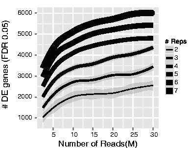
The figure below shows how the number of differentially expressed (DE) genes identified is influenced by sequencing depth and number of replicates [1]. Notice that increasing the number of replicates identifies more DE genes compared to increasing sequencing depth. This is because most of the biological variability occurs between samples. As a result, having more replicates typically yields better results than increasing sequencing depth, as it captures natural biological variability more effectively and leads to more accurate estimates of within-group variation. While increasing sequencing depth reduces technical noise, it has less impact on detecting DE genes since it doesn’t account for biological variability. Generally, a minimum sequencing depth of 20-30 million reads per sample is recommended, though successful RNA-seq experiments have been conducted with as few as 10 million reads when enough replicates are included.

NOTE

• Biological replicates represent multiple samples (i.e. RNA from different mice) representing the same sample class
• Technical replicates represent the same sample (i.e. RNA from the same mouse) but with technical steps replicated
• Usually biological variance is much greater than technical variance, so we do not need to account for technical variance to identify biological differences in expression
• Don’t spend money on technical replicates - biological replicates are much more useful

NOTE: If you are using cell lines and are unsure whether or not you have prepared biological or technical replicates, take a look at this link. This is a useful resource in helping you determine how best to set up your in-vitro experiment.

1.3.4 Differential expression analysis workflow

To model counts appropriately when performing a differential expression analysis, there are a number of software packages that have been developed for differential expression analysis of RNA-seq data. Even as new methods are continuously being developed a few tools are generally recommended as best practice, e.g. DESeq2 and EdgeR. Both these tools use the negative binomial model, employ similar methods, and typically, yield similar results. They are pretty stringent, and have a good balance between sensitivity and specificity (reducing both false positives and false negatives).

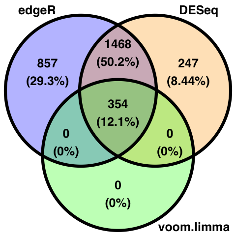
Here is a comparison of the three most highy used software packages for differential expression analysis. No single method is optimal under all circumstances, for example, limma works best when sample number is high, and edgeR and DESeq2 perform well for small sample sizes. It is also difficult to compare analysis methods due to different procedures in calculating pvalues.

We will be using DESeq2 for the DE analysis, and the analysis steps with DESeq2 are shown in the flowchart below. DESeq2 first normalizes the count data to account for differences in library sizes and RNA composition between samples. Then, we will use the normalized counts to make some plots for QC at the gene and sample level. The final step is to use the appropriate functions from the DESeq2 package to perform the differential expression analysis.

We will go in-depth into each of these steps in the following lessons, but additional details and helpful suggestions regarding DESeq2 can be found in the DESeq2 vignette. As you go through this workflow and questions arise, you can reference the vignette from within RStudio:

vignette("DESeq2")

This is very convenient, as it provides a wealth of information at your fingertips! Be sure to use this as you need during the workshop.

---

This lesson has been developed by members of the teaching team at the Harvard Chan Bioinformatics Core (HBC). These are open access materials distributed under the terms of the Creative Commons Attribution license (CC BY 4.0), which permits unrestricted use, distribution, and reproduction in any medium, provided the original author and source are credited.