Chapter 4 DGE analysis workflow
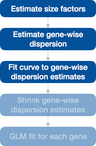
Differential expression analysis with DESeq2 involves multiple steps as displayed in the flowchart below in blue.
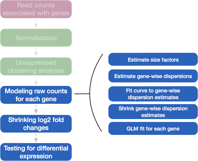
Full Workflow in DESeq2:
Load Data: Begin with raw count data (gene expression counts) and sample metadata (information about the experimental conditions).
Estimate Size Factors: Normalize counts across samples to account for differences in sequencing depth or library size, ensuring that comparisons between samples are meaningful.
Estimate Gene-Wise Dispersions: Estimate the dispersion (a measure of variability) for each gene. This represents the variance in counts that cannot be explained by differences in mean expression alone.
Fit a Global Trend for Dispersion: Model the relationship between the mean counts and the dispersion. DESeq2 allows this relationship to be fit either using a parametric model (default) or a non-parametric approach for highly variable genes.
Shrink the Gene-Wise Dispersion Estimates: Shrink the gene-wise dispersion estimates toward the global trend using an empirical Bayes approach. This step stabilizes the estimates, especially for genes with low counts, improving reliability.
Fit the Negative Binomial Model: Use the final shrunken gene-wise dispersion estimates to fit a negative binomial model for each gene. This model captures the counts’ variability and provides estimates of log-fold changes in gene expression between conditions.
Shrink the Log-Fold Changes: Optionally shrink the log-fold changes using a regularization technique to stabilize the estimates, especially for low-expression genes.
Perform Statistical Testing: Conduct statistical tests to identify genes that are differentially expressed between conditions. DESeq2 uses a Wald test to assess the significance of the log-fold changes and provides adjusted p-values to account for multiple testing.
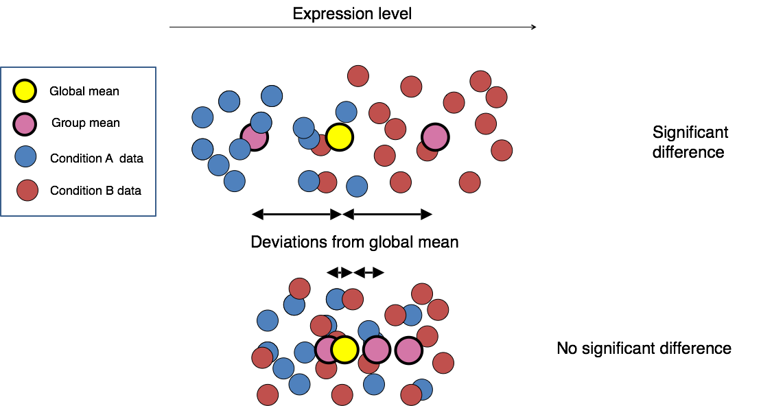
This final step in the differential expression analysis workflow of fitting the raw counts to the NB model and performing the statistical test for differentially expressed genes, is the step we care about. This is the step that determines whether the mean expression levels of different sample groups are significantly different.
The DESeq2 paper was published in 2014, but the package is continually updated and available for use in R through Bioconductor.
4.1 Running DESeq2
Prior to performing the differential expression analysis, it is a good idea to know what sources of variation are present in your data, either by exploration during the QC and/or prior knowledge. Sources of variation refer to anything that causes differences in gene expression across your samples, including biological factors (treatment, sex, age) and technical factors (batch effects, sequencing depth) and are typically factors in you metadata. These factors lead to variability in the data and can affect your ability to detect meaningful biological signals (like differential expression between treated and control samples).Once you know the major sources of variation, you can remove them prior to analysis or control for them in the statistical model by including them in your design formula.
4.1.1 Set the Design Formula
The main purpose of the design formula in DESeq2 is to specify the factors that are influencing gene expression so that their effects can be accounted for or controlled during the analysis. This allows DESeq2 to isolate the effect of the variable you’re primarily interested in while adjusting for other known sources of variation. The design formula should have all of the factors in your metadata that account for major sources of variation in your data. The last factor entered in the formula should be the condition of interest.
The design formula allows you to include multiple variables that might affect gene expression, so that DESeq2 can:
Adjust for known sources of variation (e.g., batch effects, sex, age, etc.)
Test the factor of interest (e.g., treatment) after adjusting for these confounders.
For example, let’s look at the design formula for our count matrix:
## ~sampletypeExample Suppose you have metadata that includes sex, age, and treatment as shown below:
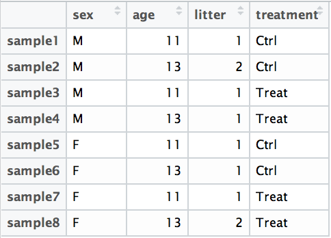
If you want to examine differences in gene expression between treatment conditions, and you know that sex and age are major sources of variation, your design formula would look like this:
design <- ~ sex + age + treatment
The design formula is specified using the tilde (~) symbol in R, with the factors of interest separated by plus (+) signs. The formula structure tells DESeq2 which known sources of variation to control for during the analysis, as well as the factor of interest to test for differential expression.
Why is this important?
By including known sources of variation (such as sex and age) in the design, DESeq2 can adjust for their effects, ensuring that any differences observed in gene expression are due to the biological condition of interest (in this case, treatment) and not confounded by other factors like sex or age. The comparison between treatment and control is still performed in the results() function, but it now accounts for these additional factors. This allows DESeq2 to isolate the effect of the variable you’re primarily interested in (e.g., treatment) while adjusting for other known sources of variation (e.g., sex, age).
To figure out the design formula, follow these steps:
- Identify your factor of interest (e.g., treatment).
- Determine any confounding variables you need to adjust for (e.g., sex, age)
- Write the formula, placing the factor of interest last.
- Explore your metadata with PCA to ensure all relevant factors are included.
Exercise points = +3
- Suppose you wanted to study the expression differences between the two age groups in the metadata shown above, and major sources of variation were sex and treatment, how would the design formula be written?
Click here to see the solution
# the default behavior of `results` is to return the comparison of the last group in the design formula, so your condition of interest should come last:

~ sex + treatment + age- Based on our Mov10 metadata dataframe, which factors could we include in our design formula?
- Ans:
Click here to see the solution
sampletype, you could also use MOVexpr, but it is
           redundant with sampletype. Sampletype is also
more descriptive.- What would you do if you wanted to include a factor in your design formula that is not in your metadata?
- Ans:
Click here to see the solution
Add the factor as an additional column in the metadata points4.1.2 MOV10 Differential Expression Analysis
Now that we understand how to specify the model in DESeq2, we can proceed with running the differential expression pipeline on the raw count data.
Running Differential Expression in Two Lines of Code To obtain differential expression results from our raw count data, we only need to run two lines of code!
First, we create a DESeqDataSet, as we did in the ‘Count normalization’ lesson, specifying the location of our raw counts and metadata, and applying our design formula:
## Create DESeq object
dds <- DESeqDataSetFromMatrix(countData = data, colData = meta, design = ~sampletype)
## Warning in DESeqDataSet(se, design = design, ignoreRank): some variables in
## design formula are characters, converting to factorsNext, we run the actual differential expression analysis with a single call to the DESeq() function. This function handles everything—from normalization to linear modeling—all in one step. During execution, DESeq2 will print messages detailing the steps being performed: estimating size factors, estimating dispersions, gene-wise dispersion estimates, modeling the mean-dispersion relationship, and statistical testing for differential expression.
## estimating size factors## estimating dispersions## gene-wise dispersion estimates## mean-dispersion relationship## final dispersion estimates## fitting model and testingBy re-assigning the result to back to the same variable name (dds), we update our DESeqDataSet object, which will now contain the results of each step in the analysis, effectively filling in the slots of our DESeqDataSet object.
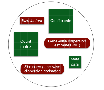
4.2 DESeq2 differential gene expression analysis workflow
With these two lines of code, we have completed the core steps in the DESeq2 differential gene expression analysis. The key steps in this workflow are summarized below:
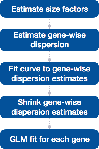
In the following sections, we will explore each step in detail to better understand how DESeq2 performs the statistical analysis and what metrics we should focus on to evaluate the quality of the results.
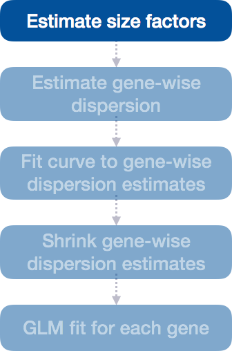
4.2.1 Step 1: Estimate size factors
The first step in the differential expression analysis is to estimate the size factors, which is exactly what we already did to normalize the raw counts.
DESeq2 will automatically estimate the size factors when performing the differential expression analysis. However, if you have already generated the size factors using estimateSizeFactors(), as we did earlier, then DESeq2 will use these values.
To normalize the count data, DESeq2 calculates size factors for each sample using the median of ratios method discussed previously in the Count normalization (Chapter 2) lesson.
4.2.1.1 MOV10 DE analysis: examining the size factors
Let’s take a quick look at size factor values we have for each sample:
## Irrel_kd_1 Irrel_kd_2 Irrel_kd_3 Mov10_kd_2 Mov10_kd_3 Mov10_oe_1 Mov10_oe_2
##  1.1224020  0.9625632  0.7477715  1.5646728  0.9351760  1.2016082  1.1205912
## Mov10_oe_3
##  0.6534987
Take a look at the total number of reads for each sample:
## Irrel_kd_1 Irrel_kd_2 Irrel_kd_3 Mov10_kd_2 Mov10_kd_3 Mov10_oe_1 Mov10_oe_2
##   22687366   19381680   14962754   32826936   19360003   23447317   21713289
## Mov10_oe_3
##   12737889
How do the numbers correlate with the size factor?
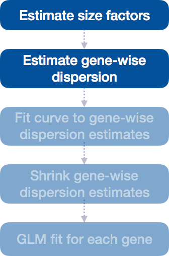
4.2.2 Step 2: Estimate gene-wise dispersion
The next step in differential expression analysis is estimating the gene-wise dispersions. Before diving into the details of how DESeq2 estimates these values, it’s important to understand what dispersion means in the context of RNA-Seq analysis.
Dispersion is a measure of variability in gene expression that cannot be explained by differences in the mean expression level alone. It captures the extra-Poisson variability observed in RNA-Seq data, where the variance tends to exceed the mean due to biological and technical factors.
What is dispersion? Dispersion is a measure of variability or spread in the data. Common measures of dispersion include variance, standard deviation, and interquartile range (IQR). However, in DESeq2, dispersion (denoted as \(\alpha\)) is specifically related to the relationship between the mean (\(\mu\)) and variance (Var) of the data:
\[Var = \mu + \alpha \mu^2\]
What does the DESeq2 dispersion represent?
Dispersion in DESeq2 reflects the variability in gene expression for a given mean count. It is inversely related to the mean and directly related to variance:
Genes with lower mean counts tend to have higher dispersion (more variability). Genes with higher mean counts tend to show lower dispersion (less variability). Dispersion estimates for genes with the same mean will differ based on their variance, making dispersion an important metric for understanding the variability in expression across biological replicates.
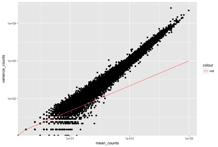
The plot below shows the relationship between mean and variance in gene expression. Each black dot represents a gene. Notice that for genes with higher mean counts, the variance can be predicted more reliably. However, for genes with low mean counts, the variance has a wider spread, and the dispersion estimates tend to vary more.
How does the dispersion relate to our model?
To accurately model sequencing counts, it’s crucial to estimate within-group variation (variation between replicates within the same experimental group) for each gene. However, with small sample sizes (e.g., 3-6 replicates per group), gene-specific estimates of variation can be unreliable, particularly for genes with similar mean counts but different dispersions.
To address this, DESeq2 shares information across genes with similar expression levels to improve dispersion estimates. This is done through a process called shrinkage, which assumes that genes with similar mean expression tend to have similar dispersion. By borrowing strength from the entire dataset, DESeq2 produces more accurate estimates of variation.
How DESeq2 Models Dispersion Using the Negative Binomial Distribution DESeq2 uses the negative binomial (NB) distribution to model count data in RNA-Seq experiments. The NB distribution accounts for the overdispersion observed in real biological data, where the variance tends to be greater than the mean. The two key parameters of the NB distribution are the mean expression level and the dispersion.
For each gene \(i\), the observed count \(Y_{ij}\) in sample \(j\) is modeled as:
\[ Y_{ij} \sim \text{NB}\left(\mu_{ij}, \alpha_{i}\right) \] Where:
\(Y_{ij}\) is the observed count for gene \(i\) in sample \(j\)
\(\mu_{ij}\) = is the expected normalized count for gene \(i\) in sample \(j\) and is equal to the \(sizeFactor_{j}\) \(q_{i}\) where \(q_{i}\) is the true expression level of gene \(i\)
\(\alpha_{i}\) is the dispersion parameter for gene \(i\)
\(sizeFactor_{j}\) normalizes the counts for differences in sequencing depth across samples
This model captures both the variability in sequencing depth (through the size factor) and the biological variability across genes (through the dispersion).
Estimating the dispersion for each gene separately:
The first step in estimating dispersion is to get the dispersion estimates for each gene. The dispersion for each gene is estimated using maximum likelihood estimation (MLE). MLE can be thought about as finding the value of \(\alpha_{i}\) that makes the observed counts \(Y_{ij}\) most likely under the model. The dispersion parameter for each gene \(\alpha_{i}\) represents the extra-Poisson variability in the data, which accounts for biological and technical variability not explained by the mean expression level. Estimating this accurately is crucial for modeling the count data and identifying differentially expressed genes and accounts for how much variability exceeds the mean.
Dispersion is a measure of spread or variability in the data. DESeq2 uses a specific measure of dispersion (α) related to the mean (μ) and variance of the data: \(Var = μ + α*μ^2\). For genes with moderate to high count values, the square root of dispersion will be equal to the coefficient of variation (σ/ μ). So 0.01 dispersion means 10% variation around the mean expected across biological replicates.
We can make a rough estimate of the gene-wise dispersions using this formula. We know that:
\[Var(Y_{ij}) = {\mu_{ij} + \alpha_{i}}{\mu_{ij}^2}\]
So the dispersion is equal to: \[\alpha_{i} = \frac{Var(Y_{ij}) - \mu_{ij}}{\mu_{ij}^2}\] For genes with moderate to high counts, the term \(\alpha_{i} \mu^2\) dominates the variance, so:
\[Var(Y_{ij}) \approx \alpha_{i} \mu_{ij}^2\] and the standard deviation is:
\[\sqrt{Var(Y_{ij})} = \sigma_{ij} \approx \sqrt{\alpha_{i} \mu_{ij}^2} = \sqrt{\alpha_{i}} \mu_{ij}\] and the square root of the dispersion is approximately the coefficient of variation:
\[\sqrt{\alpha_{i}} \approx \frac{\sigma_{ij}}{\mu_{ij}}\]
Which is equal to the coefficient of variation (CV) for genes with moderate to high counts. The CV is a measure of relative variability, calculated as the standard deviation divided by the mean. For genes with low counts, the dispersion is more complex and depends on the mean expression level.
4.2.3 Step 3: Fit Curve to Gene-Wise Dispersion Estimates
Once DESeq2 has estimated the initial gene-wise dispersions (\(\alpha_{i}\)) using maximum likelihood, the next step is to fit a global trend to model how dispersion typically changes as a function of the mean expression (\(\mu_{i}\)) across all genes and samples. This allows DESeq2 to borrow strength from the overall dataset and stabilize the dispersion estimates, especially for genes with low counts or high variability.
Fitting the Global Dispersion Trend
The global trend models the general relationship between gene expression and dispersion. In RNA-Seq data, genes with low mean expression typically show greater variability (higher dispersion), while genes with high expression tend to be more stable (lower dispersion). By fitting this trend, DESeq2 smooths out gene-specific variability and provides better estimates of dispersion for all genes.
The global trend represents the expected dispersion value for genes at different expression levels. While individual genes may have varying biological variability, there is a consistent relationship across all genes between expression and dispersion. Fitting a curve to this data ensures that the dispersion estimates are more accurate.
Why is this important?
Lowly expressed genes tend to show more variability across replicates, making dispersion estimates noisy.
Highly expressed genes have more stable counts, with lower dispersion.
By fitting a curve to capture this general trend, DESeq2 ensures that genes with low counts or high variability have more reliable dispersion estimates.
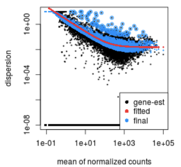
Visual representation of the global dispersion trend:
The red line in the plot below shows the global trend, which represents the expected dispersion value for genes of a given expression level. Each black dot corresponds to a gene, plotted with its mean expression and initial dispersion estimate from maximum likelihood estimation (Step 2).
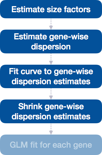
4.2.4 Step 4: Shrinking Gene-Wise Dispersion Estimates Toward the Global Trend
After fitting the global trend, DESeq2 applies empirical Bayes shrinkage to the individual gene-wise dispersion estimates, pulling them toward the curve. Empirical Bayes shrinkage is a statistical technique used to stabilize parameter estimates by borrowing information across the entire dataset. This process helps reduce the noise in the estimates, particularly for genes with low counts.
Low-count genes with more uncertain dispersion estimates are pulled closer to the global trend.
Genes with higher counts or more reliable estimates will be shrunk less.
Why is shrinkage important?
Shrinkage improves the reliability of dispersion estimates by making them more stable, especially for genes with low or moderate counts, where the estimates are typically noisier. This ensures that dispersion estimates are not overly influenced by random fluctuations and are more accurate for downstream differential expression testing.
Shrinkage is crucial for reducing false positives in differential expression analysis. Genes with low or moderate dispersion estimates are pulled up toward the curve, making the estimates more reliable for subsequent model fitting and differential expression testing.
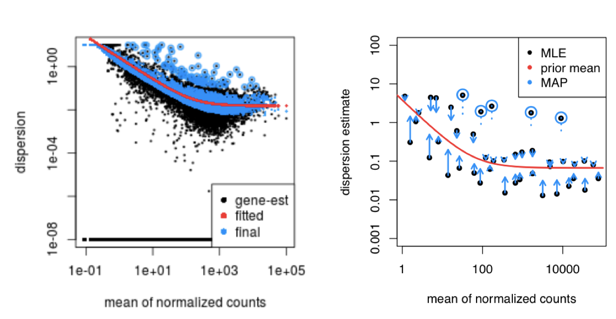
Even dispersions slightly above the curve are shrunk toward the trend for consistency. However, genes with extremely high dispersion values (potential outliers) are typically not shrunk. These genes may exhibit higher variability due to biological or technical reasons, and shrinking them could lead to false positives. These outlier genes are highlighted by blue circles in the plot below:
By shrinking the estimates toward the fitted curve, DESeq2 ensures that the final dispersion estimates are more stable and accurate for differential expression testing.
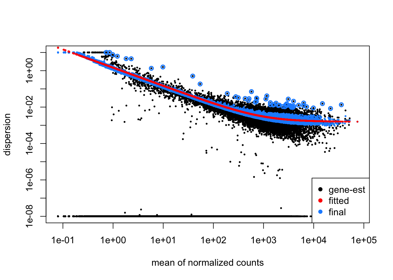
Assessing Model Fit with Dispersion Plots
After shrinkage, it’s important to assess how well the model fits the data. The dispersion plot shows gene-wise dispersions relative to the global trend. Ideally, most genes should scatter around the curve, with dispersions decreasing as mean expression increases.
If you notice unusual patterns, such as a cloud of points far from the curve, this could indicate data quality issues (e.g., outliers, contamination, or problematic samples). Using DESeq2’s plotDispEsts() function helps visualize the fit of the model and the extent of shrinkage across genes.
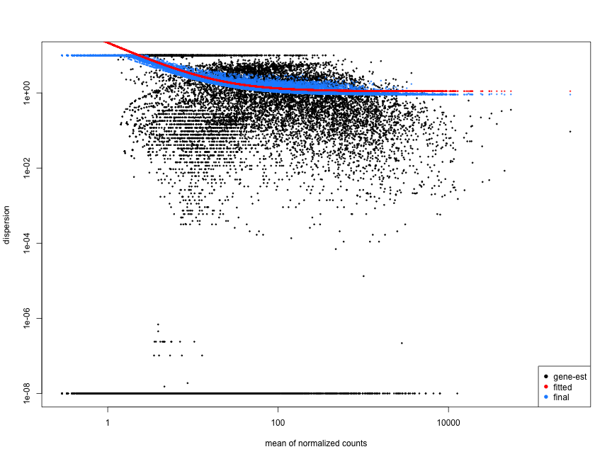
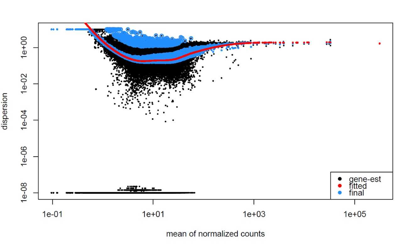
Examples of Problematic Dispersion Plots:
Below are examples of worrisome dispersion plots that suggest potential issues with data quality or fit:
 ### MOV10 Differential Expression Analysis: Exploring Dispersion Estimates
Now, let’s explore the dispersion estimates for the MOV10 dataset:
Since we have a small sample size, for many genes we see quite a bit of shrinkage. Do you think our data are a good fit for the model?