Chapter 3 Spatial Analysis
3.1 Data
library(tidyverse); library(sf); library(cowplot); library(magrittr)


list <- read.csv("./_data/us_abbrev.csv", stringsAsFactors = F) %>%
  mutate(state = trimws(state),
         STATE = trimws(STATE))

nsduh <- read.csv("./_data/NSDUH_final2.csv", stringsAsFactors = F) %>%
  dplyr::select(outcome, year_pair, state, estimate) %>%
  mutate(outcome = ifelse(outcome=="Needing But Not Receiving Treatment for Substance Use at a Specialty Facility in the Past Year (2015 onward)", "Needing But Not Receiving Treatment for Substance Use at a Specialty Facility in the Past Year (through 2014)", outcome)) %>%
  spread(outcome, estimate) %>%
  dplyr::rename(heroin = `Heroin Use in the Past Year`,
         tx_su = `Needing But Not Receiving Treatment for Substance Use at a Specialty Facility in the Past Year (through 2014)`,
         tx_mental = `Received Mental Health Services in the Past Year`,
         mental = `Serious Mental Illness in the Past Year`) %>%
  dplyr::select(year_pair, state, heroin, tx_su, tx_mental, mental) %>%
  mutate(year = as.numeric(str_sub(year_pair,1,4))) %>%
  inner_join(list, by = "state")

data <- read.csv("./_data/Cleaned_Final_Dataset_2018_7-2-20.csv", stringsAsFactors = F) %>%
  dplyr::rename(County.Code = county_code) %>%
  separate(county_name, c("County", "STATE"), sep = ", ") %>%
  mutate_all(.funs = ~ifelse(.==-999,NA,.)) %>%
  dplyr::select(-c(X, state, #County, STATE,
                heroin_deaths, cocaine_deaths, meth_deaths,
                #heroin_crude_death_rate, cocaine_crude_death_rate, meth_crude_death_rate,
                next_year_synthetic_opioid_death_rate, two_year_out_synthetic_opioid_death_rate)) %>%
  inner_join(nsduh, by = c("STATE", "year"))

usa.sf <- st_read("./_data/GIS/tl_2017_us_county/tl_2017_us_county.shp",  stringsAsFactors = F) %>%
  #filter(STATEFP=="01") %>%
  filter(STATEFP!="02", STATEFP!="15", STATEFP!="60", STATEFP!="66", STATEFP!="69", STATEFP!="72", STATEFP!="78") %>%
  mutate(County.Code = as.numeric(GEOID),
         STATEFP = as.numeric(STATEFP)) %>%
  left_join(read_excel("./_data/fp_codes.xlsx") %>%
              dplyr::rename(STATEFP = `Numeric code`), by = "STATEFP")

dat.full <- usa.sf %>%
  dplyr::select(County.Code, loc) %>%
  inner_join(data, by="County.Code")
3.2 Spatial Analysis
library(spdep)
library(tmap)

usa.sp <- as(usa.sf, "Spatial")

map.sf <- usa.sf %>%
  dplyr::select(County.Code, loc) %>%
  inner_join(data %>% distinct(County.Code), by="County.Code")

nb <- poly2nb(map.sf)
self <- nb2listw(include.self(nb))

breaks <- c(-Inf, -2.58, -1.96, -1.65, 1.65, 1.96, 2.58, Inf)
labels <- c("Cold spot: 99% confidence", "Cold spot: 95% confidence", "Cold spot: 90% confidence", "County Not significant","Hot spot: 90% confidence", "Hot spot: 95% confidence", "Hot spot: 99% confidence")

usa.getis <- dat.full %>%
  st_set_geometry(NULL) %>%
  nest(-year) %>%
  mutate(LISA = map(.x = data, .f = ~localG(.x$synthetic_opioid_crude_death_rate, self)),
         clust_LISA = map(.x = LISA, .f = ~cut(.x, include.lowest = TRUE, breaks = breaks, labels = labels))) %>%
  unnest() %>%
  dplyr::select(County.Code, year, LISA, clust_LISA)

dat.full.getis <- usa.sf %>%
  dplyr::select(County.Code, loc) %>%
  inner_join(usa.getis, by="County.Code")

(fig2a <- dat.full.getis %>%
    ggplot() +
    geom_sf(aes(fill=clust_LISA), col = NA) +
    geom_sf(data = dat.full.getis %>% summarise(n = n()), fill = NA) +
    scale_fill_brewer(name="Cluster", palette = "RdBu", direction=-1) +
    facet_wrap(.~year, ncol = 3) +
    theme_bw() +
    theme(legend.position = c(1, 0),
          legend.justification = c(1, 0))
)

ggsave("./_out/fig2a.png", fig2a, height = 8, width = 13)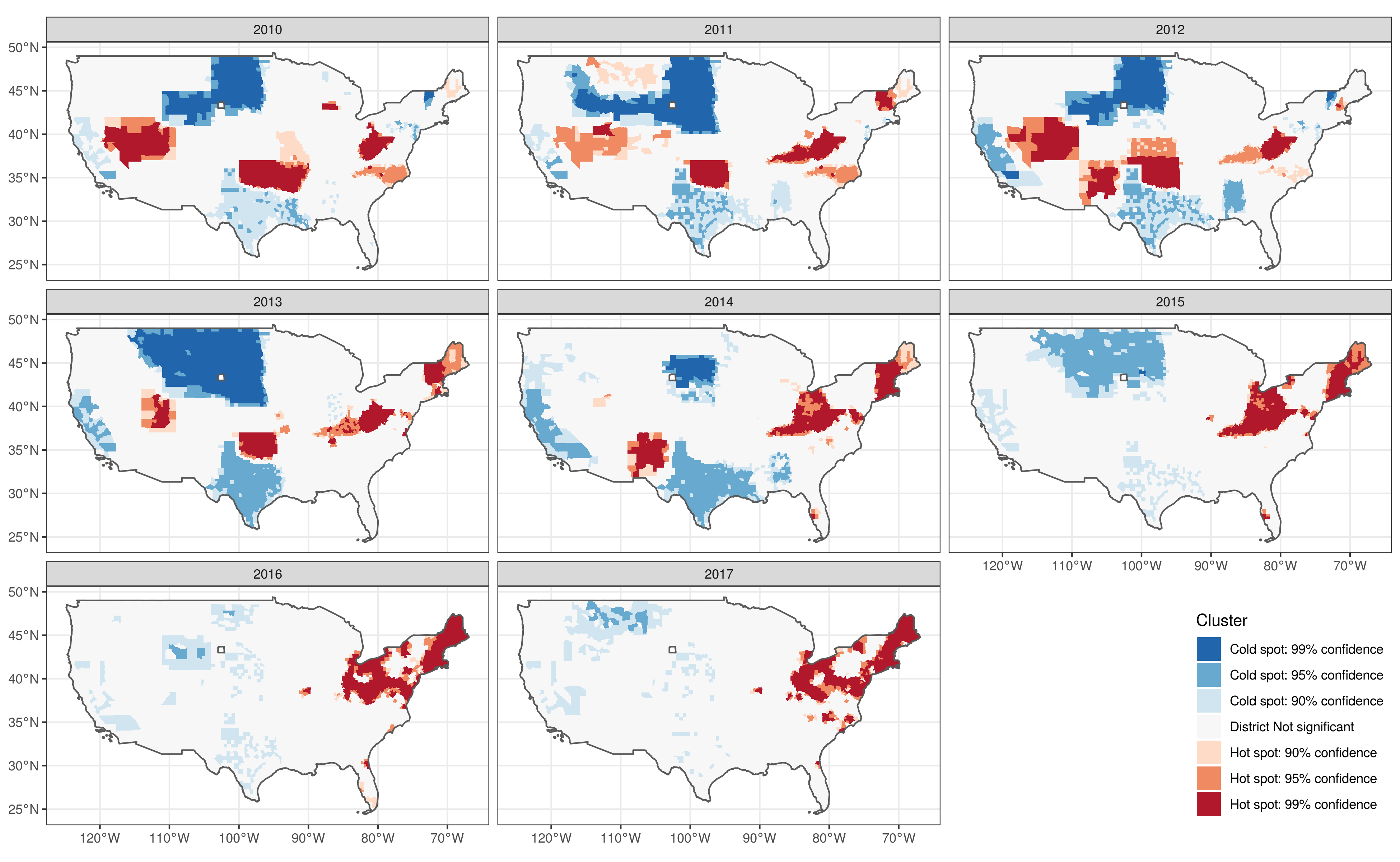
3.3 Stability
a <- dat.full.getis %>%
  st_set_geometry(NULL) %>%
  select(-LISA) %>%
  mutate(clust = clust_LISA,
         clust_LISA = as.numeric(clust_LISA))

# Correlation
library(GGally)
a %>%
  spread(year, clust_LISA) %>%
  select(-County.Code, -loc) %>%
  ggcorr(label = T)

# Kendals W
library(synchrony)
library(purrr)

b <- a %>%
  #group_by(County.Code, loc) %>%
  nest() %>%
  expand_grid(year1 = 2010:2017) %>%
  expand_grid(year2 = 2010:2017) %>%
  filter(year1 >= year2) %>%
  filter(year1 != year2) %>%
  mutate(subset = pmap(.l = list(x=data, y=year1, z=year2), .f = function(x, y, z) filter(x, year==y | year==z)),
         reshape = map(.x = subset, .f = ~spread(.x, year, clust_LISA) %>% select(-County.Code, -loc)),
         w = map(.x = reshape, .f = ~kendall.w(.x, nrands=99, type = 2)), #change to rands=999 for paper
         w.d = map(.x = w, .f = ~as.data.frame(as.list(.x)[-6])))

c <- b %>%
  select(year1, year2, w.d) %>%
  unnest()

# Coldspot

c.b <- a %>%
  # ===============
  group_by(County.Code, loc) %>%
  mutate(i = min(clust_LISA)) %>%
  filter(i<4) %>%
  ungroup() %>%
  # ===============
  nest() %>%
  expand_grid(year1 = 2010:2017) %>%
  expand_grid(year2 = 2010:2017) %>%
  filter(year1 >= year2) %>%
  filter(year1 != year2) %>%
  mutate(subset = pmap(.l = list(x=data, y=year1, z=year2), .f = function(x, y, z) filter(x, year==y | year==z)),
         reshape = map(.x = subset, .f = ~spread(.x, year, clust_LISA) %>% select(-County.Code, -loc)),
         w = map(.x = reshape, .f = ~kendall.w(.x, nrands=99, type = 2)), #change to rands=999 for paper
         w.d = map(.x = w, .f = ~as.data.frame(as.list(.x)[-6])))

c.c <- c.b %>%
  select(year1, year2, w.d) %>%
  unnest()

### Hotspot

h.b <- a %>%
  # ===============
  group_by(County.Code, loc) %>%
  mutate(i = max(clust_LISA)) %>%
  filter(i>4) %>%
  ungroup() %>%
  # ===============
  nest() %>%
  expand_grid(year1 = 2010:2017) %>%
  expand_grid(year2 = 2010:2017) %>%
  filter(year1 >= year2) %>%
  filter(year1 != year2) %>%
  mutate(subset = pmap(.l = list(x=data, y=year1, z=year2), .f = function(x, y, z) filter(x, year==y | year==z)),
         reshape = map(.x = subset, .f = ~spread(.x, year, clust_LISA) %>% select(-County.Code, -loc)),
         w = map(.x = reshape, .f = ~kendall.w(.x, nrands=99, type = 2)), #change to rands=999 for paper
         w.d = map(.x = w, .f = ~as.data.frame(as.list(.x)[-6])))

h.c <- h.b %>%
  select(year1, year2, w.d) %>%
  unnest()

# Plots

f1 <- c %>%
  ggplot(aes(x = year1, y = year2, fill = w.corrected)) +
  geom_tile() +
  scale_y_continuous(trans="reverse", breaks = c(2010:2017), expand = c(0,0)) +
  scale_x_continuous(breaks = c(2010:2017), expand = c(0,0)) +
  scale_fill_viridis_c(direction = -1, lim = c(0,1)) +
  coord_equal() +
  geom_label(aes(label = round(w.corrected, 2), col = ifelse(w.corrected>.55,"a","b")), label.size = NA) +
  scale_color_manual(values = c("white", "black")) +
  guides(color="none") +
  ggtitle("Overall") +
  labs(x = "Clusters at target year", y = "Clusters at starting year") +
  theme_minimal()

f2 <- c.c %>%
  ggplot(aes(x = year1, y = year2, fill = w.corrected)) +
  geom_tile() +
  scale_y_continuous(trans="reverse", breaks = c(2010:2017), expand = c(0,0)) +
  scale_x_continuous(breaks = c(2010:2017), expand = c(0,0)) +
  scale_fill_viridis_c(direction = -1, lim = c(0,1)) +
  coord_equal() +
  geom_label(aes(label = round(w.corrected, 2), col = ifelse(w.corrected>.55,"a","b")), label.size = NA) +
  scale_color_manual(values = c("black")) +
  guides(color="none") +
  ggtitle("Coldspots") +
  labs(x = "Clusters at target year", y = "Clusters at starting year") +
  theme_minimal()

f3 <- h.c %>%
  ggplot(aes(x = year1, y = year2, fill = w.corrected)) +
  geom_tile() +
  scale_y_continuous(trans="reverse", breaks = c(2010:2017), expand = c(0,0)) +
  scale_x_continuous(breaks = c(2010:2017), expand = c(0,0)) +
  scale_fill_viridis_c(direction = -1, lim = c(0,1)) +
  coord_equal() +
  geom_label(aes(label = round(w.corrected, 2), col = ifelse(w.corrected>.55,"a","b")), label.size = NA) +
  scale_color_manual(values = c("white", "black")) +
  guides(color="none") +
  ggtitle("Hotspots") +
  labs(x = "Clusters at target year", y = "Clusters at starting year") +
  theme_minimal()

library(cowplot)
fig3 <- plot_grid(f1, plot_grid(f2,f3, ncol = 1), ncol = 2)

ggsave("./_out/fig3.png", fig3, height = 8, width = 13)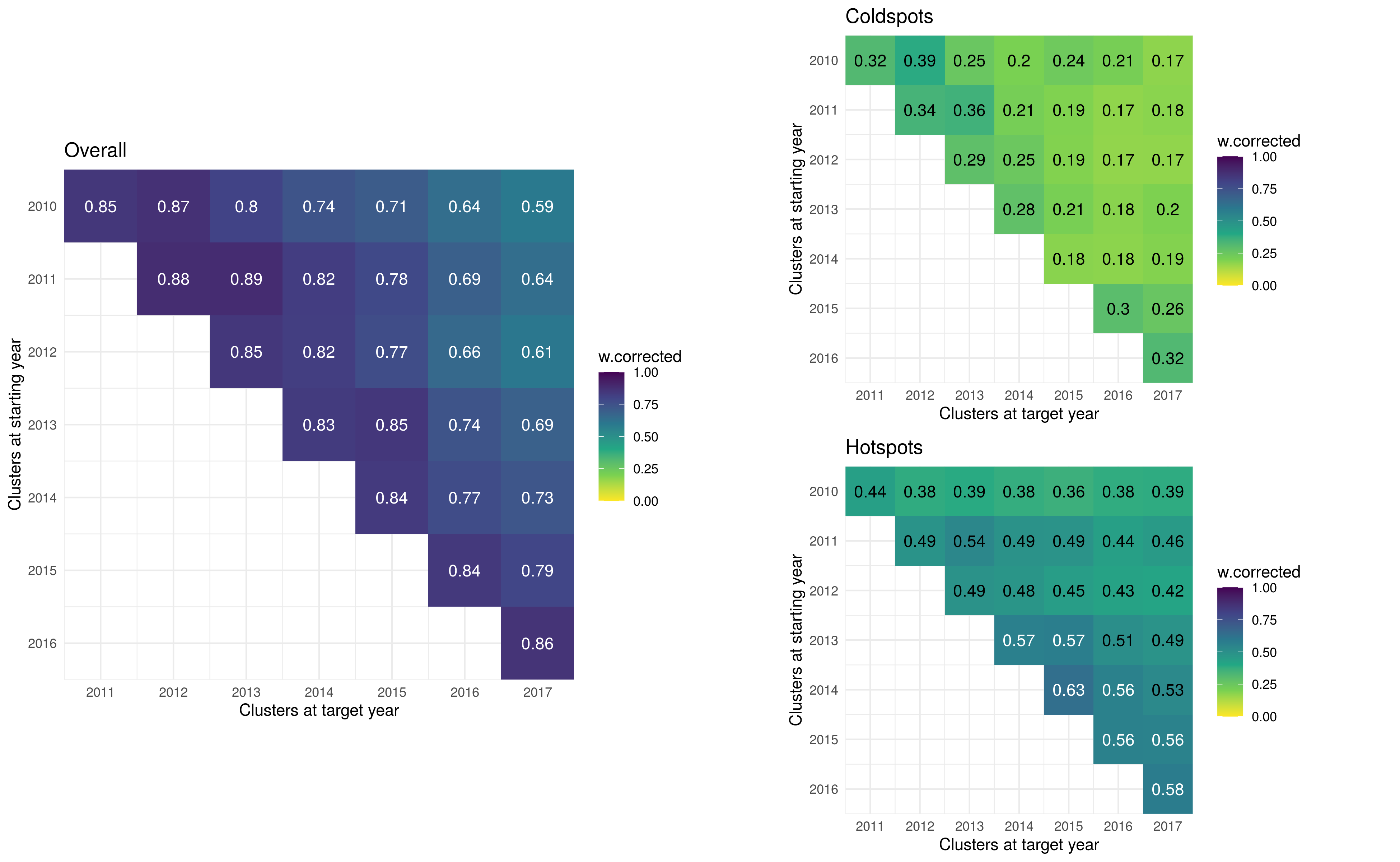
3.4 Stable clusters
library(ggthemes)
sa <- a %>%
spread(year, clust_LISA) %>%
mutate(pattern = paste0(`2010`,`2011`,`2012`,`2013`,`2014`,`2015`,`2016`,`2017`))
epiDisplay::tab1(sa$pattern, sort.group = "decreasing")
sa %>%
group_by(pattern) %>%
count() %>%
filter(n>10) %>%
ggplot(aes(x = fct_reorder(pattern,-n), y = n)) +
geom_col()
a %>%
inner_join(sa %>% dplyr::select(County.Code, pattern), by = "County.Code") %>%
mutate(n4 = str_count(pattern, "4")) %>%
#filter(n4<2) %>%
#filter(pattern != "44444444") %>%
group_by(County.Code) %>%
mutate(ord = sum(clust_LISA)) %>%
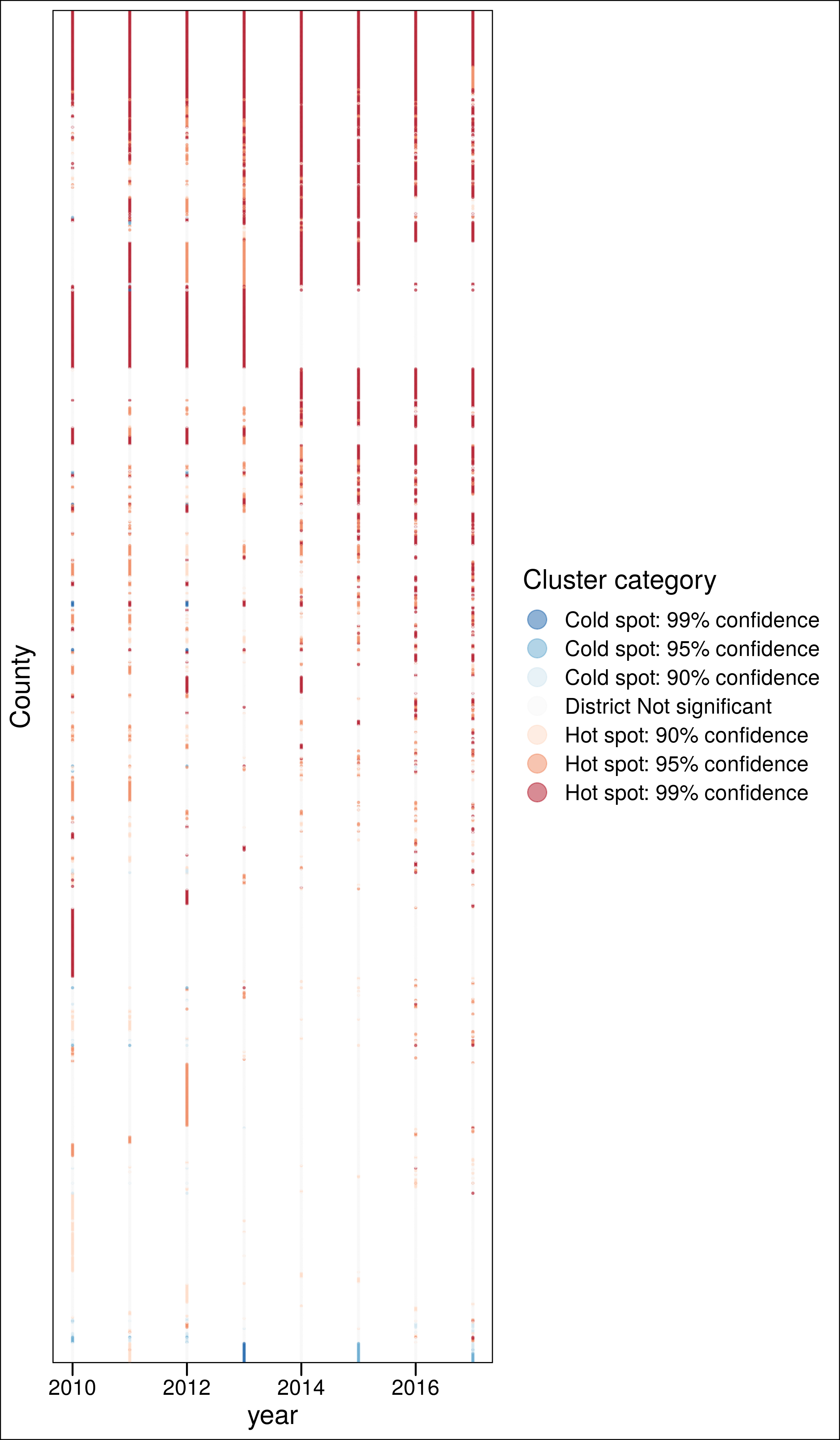
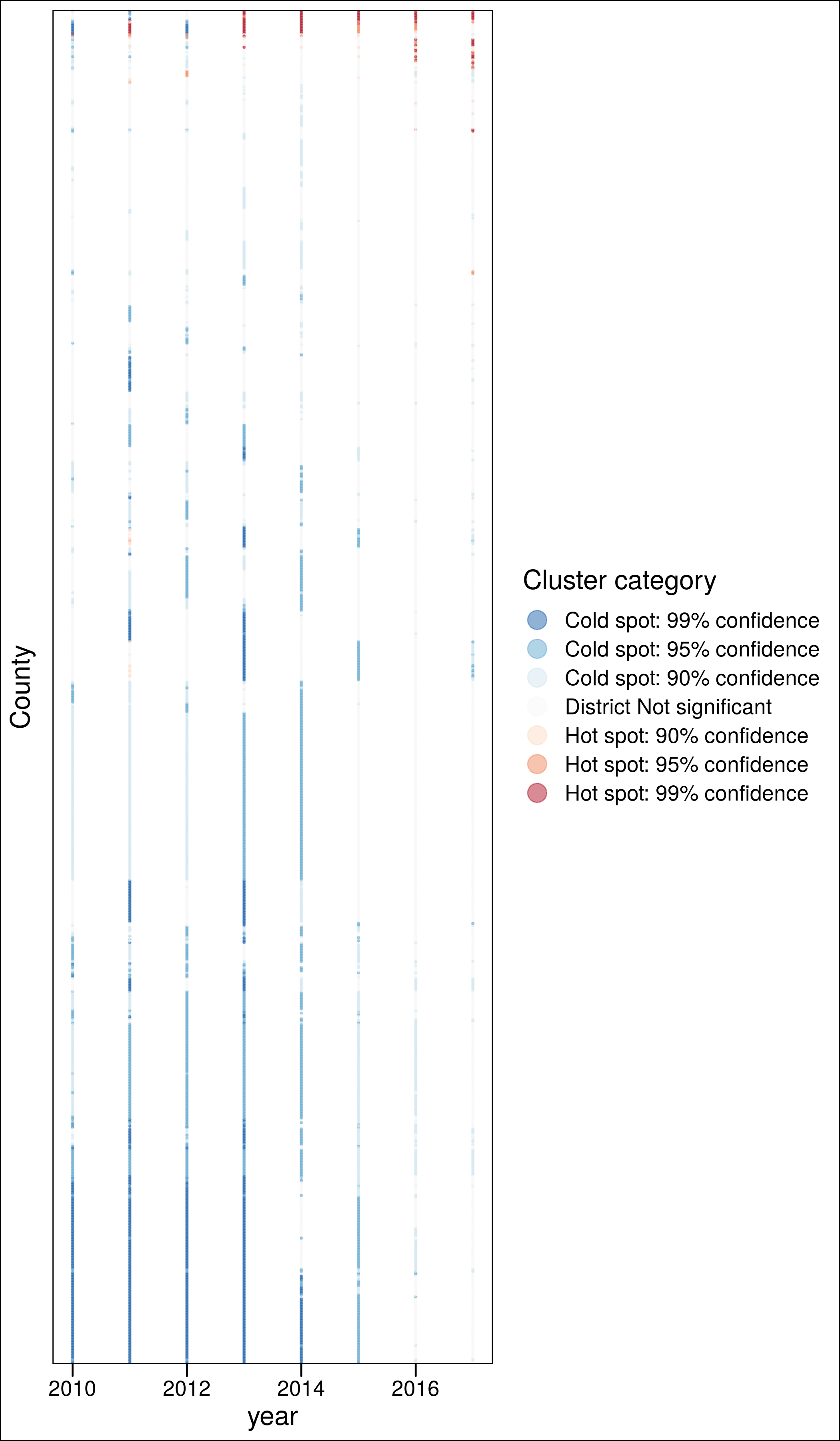
ggplot(aes(x = year, y = fct_reorder(as.factor(County.Code), ord), color = clust)) +
geom_point(alpha = .5, size = .3) +
scale_color_brewer(palette = "RdBu", direction = -1) +
labs(y = "County",
#caption = "Consistent (>4y) non-significant clusters excluded",
color = "Cluster category") +
theme_base() +
guides(colour = guide_legend(override.aes = list(size=5))) +
theme(axis.text.y = element_blank(),
axis.ticks.y = element_blank()) +
ggsave("./_out/panel.png", height = 12)
# Coldspots
a %>%
# ===============
group_by(County.Code, loc) %>%
mutate(i = min(clust_LISA)) %>%
filter(i<4) %>%
# ==============
inner_join(sa %>% dplyr::select(County.Code, pattern), by = "County.Code") %>%
mutate(n4 = str_count(pattern, "4")) %>%
#filter(n4<2) %>%
#filter(pattern != "44444444") %>%
group_by(County.Code) %>%
mutate(ord = sum(clust_LISA)) %>%
ggplot(aes(x = year, y = fct_reorder(as.factor(County.Code), ord), color = clust)) +
geom_point(alpha = .5, size = .3) +
scale_color_brewer(palette = "RdBu", direction = -1) +
labs(y = "County",
#caption = "Consistent (>4y) non-significant clusters excluded",
color = "Cluster category") +
theme_base() +
guides(colour = guide_legend(override.aes = list(size=5))) +
theme(axis.text.y = element_blank(),
axis.ticks.y = element_blank()) +
ggsave("./_out/panel_c.png", height = 12)
# Hotspot
a %>%
# ===============
group_by(County.Code, loc) %>%
mutate(i = max(clust_LISA)) %>%
filter(i>4) %>%
# ==============
inner_join(sa %>% dplyr::select(County.Code, pattern), by = "County.Code") %>%
mutate(n4 = str_count(pattern, "4")) %>%
#filter(n4<2) %>%
#filter(pattern != "44444444") %>%
group_by(County.Code) %>%
mutate(ord = sum(clust_LISA)) %>%
ggplot(aes(x = year, y = fct_reorder(as.factor(County.Code), ord), color = clust)) +
geom_point(alpha = .5, size = .3) +
scale_color_brewer(palette = "RdBu", direction = -1) +
labs(y = "County",
#caption = "Consistent (>4y) non-significant clusters excluded",
color = "Cluster category") +
theme_base() +
guides(colour = guide_legend(override.aes = list(size=5))) +
theme(axis.text.y = element_blank(),
axis.ticks.y = element_blank()) +
ggsave("./_out/panel_h.png", height = 12)3.4.1 Overall
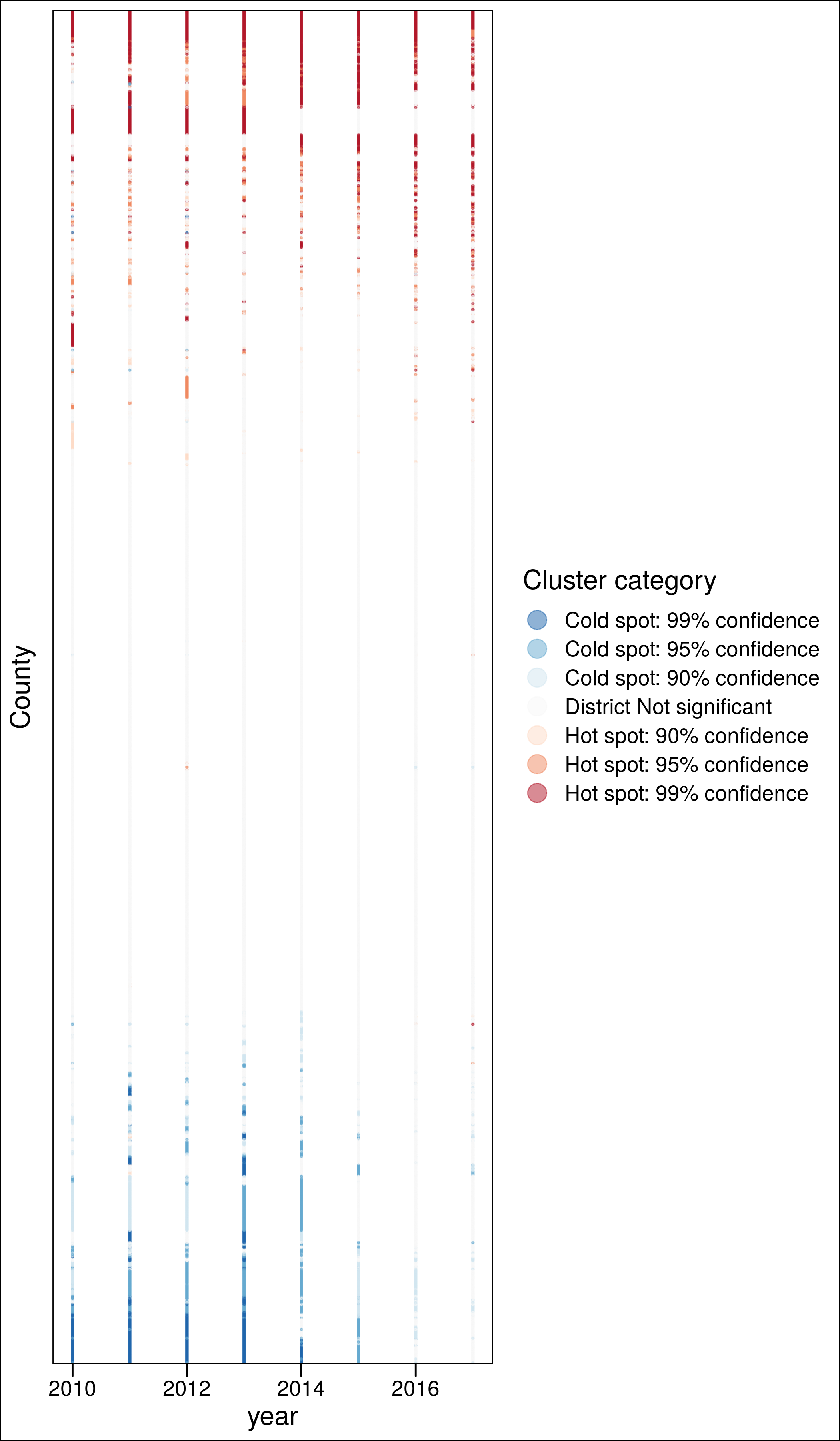
3.4.2 Coldspots
Counties with at least one year as coldspot
3.4.3 Hotspots
Counties with at least one year as hotspot