Chapter 5 MODEL
5.1 LIBRARIES
rm(list=ls())
library(tidyverse); library(epiDisplay); library(lubridate)
library(spdep); library(sf); library(sp)
library(maptools); library(rgdal); library(INLA);
library(MatrixModels); library(graph); library(Rgraphviz)
library(readxl)
library(pubh); library(huxtable); library(janitor); library(broom)

#OPTIONS
options('huxtable.knit_print_df_theme' = theme_article)
options('huxtable.autoformat_number_format' = list(numeric = "%5.2f"))
## Sourcing https://gist.githubusercontent.com/gcarrascoe/89e018d99bad7d3365ec4ac18e3817bd/raw/a288c6e1035c1c0aca2af1e2376d84f5c14a6164/CLIM_MAL_v5_functions.R## SHA-1 hash of file is b8efb09d243c1f5bfd5e4d069bbe3d7b43ec8d51## Loading required package: viridisLite5.2 ADMINISTRATIVE AND SPATIAL DATA
list <- read.csv("./_data/us_abbrev.csv", stringsAsFactors = F) %>%
  mutate(state = trimws(state),
         STATE = trimws(STATE))

nsduh <- read.csv("./_data/NSDUH_final2.csv", stringsAsFactors = F) %>%
  dplyr::select(outcome, year_pair, state, estimate) %>%
  mutate(outcome = ifelse(outcome=="Needing But Not Receiving Treatment for Substance Use at a Specialty Facility in the Past Year (2015 onward)", "Needing But Not Receiving Treatment for Substance Use at a Specialty Facility in the Past Year (through 2014)", outcome)) %>%
  spread(outcome, estimate) %>%
  dplyr::rename(heroin = `Heroin Use in the Past Year`,
         tx_su = `Needing But Not Receiving Treatment for Substance Use at a Specialty Facility in the Past Year (through 2014)`,
         tx_mental = `Received Mental Health Services in the Past Year`,
         mental = `Serious Mental Illness in the Past Year`) %>%
  dplyr::select(year_pair, state, heroin, tx_su, tx_mental, mental) %>%
  mutate(year = as.numeric(str_sub(year_pair,1,4))) %>%
  inner_join(list, by = "state")

data <- read.csv("./_data/Cleaned_Final_Dataset_2018_7-2-20.csv", stringsAsFactors = F) %>%
  dplyr::rename(County.Code = county_code) %>%
  separate(county_name, c("County", "STATE"), sep = ", ") %>%
  mutate_all(.funs = ~ifelse(.==-999,NA,.)) %>%
  dplyr::select(-c(X, state, #County, STATE,
                heroin_deaths, cocaine_deaths, meth_deaths,
                #heroin_crude_death_rate, cocaine_crude_death_rate, meth_crude_death_rate,
                next_year_synthetic_opioid_death_rate, two_year_out_synthetic_opioid_death_rate)) %>%
  inner_join(nsduh, by = c("STATE", "year"))

usa.sf <- st_read("./_data/GIS/tl_2017_us_county/tl_2017_us_county.shp",  stringsAsFactors = F) %>%
  #filter(STATEFP=="01") %>%
  filter(STATEFP!="02", STATEFP!="15", STATEFP!="60", STATEFP!="66", STATEFP!="69", STATEFP!="72", STATEFP!="78") %>%
  mutate(County.Code = as.numeric(GEOID),
         STATEFP = as.numeric(STATEFP)) %>%
  left_join(read_excel("./_data/fp_codes.xlsx") %>%
              dplyr::rename(STATEFP = `Numeric code`), by = "STATEFP")

# Variable Names
#paste(colnames(dat.N), collapse=" + ")
5.3 GEGRAPHIC STRATA
5.3.1 NorthEast
# -----------------
# Data
# -----------------
usa.N <- usa.sf %>%
  filter(loc == "N") %>%
  mutate(index = 1:n(),
         index2 = index)

nb.map.N <- poly2nb(usa.N)
#nb2INLA("map.graph.N",nb.map.N)

index.N <- usa.N %>%
  dplyr::select(County.Code, ALAND, index, index2) %>%
  st_set_geometry(NULL)

dat.N <- data %>%
  inner_join(index.N, by="County.Code") %>%
  inner_join(n.neighbors(nb.map.N), by = "index") %>%
  dplyr::select(-County.Code, -index2) %>%
  mutate(urbanicity = factor(urbanicity),
         synthetic_opioid_crude_death_rate = as.character(synthetic_opioid_crude_death_rate),
         population = as.character(population),
         synthetic_opioid_deaths = as.character(synthetic_opioid_deaths),
         year = as.character(year),
         index = as.character(index)) %>%
  mutate_if(is.numeric, scale_this) %>%
  mutate(synthetic_opioid_crude_death_rate = as.numeric(synthetic_opioid_crude_death_rate),
         population = as.numeric(population),
         synthetic_opioid_deaths = floor(as.numeric(synthetic_opioid_deaths)),
         year = as.numeric(year),
         index = as.numeric(index))

n.N<-nrow(dat.N)

# -----------------
# Formula
# -----------------

N<-c(
  # NULL
  formula = synthetic_opioid_deaths ~ 1,
  # Spatio-temporal only
  formula = synthetic_opioid_deaths ~ 1 + f(index, model = "besag", graph = "map.graph.N") + f(year, model = "rw1"),
  # Healthcare system
  formula = synthetic_opioid_deaths ~ 1 + urgent_care + proportion_uninsured + buprenorphine_provider_waivers,
  # Healthcare system spatial
  formula = synthetic_opioid_deaths ~ 1 + urgent_care + proportion_uninsured + buprenorphine_provider_waivers + f(index, model = "besag", graph = "map.graph.N") + f(year, model = "rw1"),
  #Socio-economic
  formula = synthetic_opioid_deaths ~ 1 + proportion_male + proportion_black + proportion_american_indian_alaska_native + proportion_asian + proportion_native_hawaiian_pacific_islander + proportion_high_school_or_greater + proportion_bachelors_or_greater + proportion_poverty + unemployment_rate + mean_household_income + proportion_homeowners_35perc_income + proportion_renters_35perc_income + urbanicity,
  #Socio-economic spatial
  formula = synthetic_opioid_deaths ~ 1 + proportion_male + proportion_black + proportion_american_indian_alaska_native + proportion_asian + proportion_native_hawaiian_pacific_islander + proportion_high_school_or_greater + proportion_bachelors_or_greater + proportion_poverty + unemployment_rate + mean_household_income + proportion_homeowners_35perc_income + proportion_renters_35perc_income + urbanicity + f(index, model = "besag", graph = "map.graph.N") + f(year, model = "rw1"),
  # Drug market
  formula = synthetic_opioid_deaths ~ 1 + NFLIS + opioid_prescriptions_per_100 + police_violence + road_access,
  # Drug market spatial
  formula = synthetic_opioid_deaths ~ 1 + NFLIS + opioid_prescriptions_per_100 + police_violence + road_access + f(index, model = "besag", graph = "map.graph.N") + f(year, model = "rw1"),
  # Individual susceptibility/prevalence of drug use
  formula = synthetic_opioid_deaths ~ 1 + hep_c_mortality_rate + heroin_crude_death_rate + cocaine_crude_death_rate + meth_crude_death_rate + heroin + tx_su + tx_mental + mental,
  # Individual susceptibility/prevalence of drug use spatial
    formula = synthetic_opioid_deaths ~ 1 + hep_c_mortality_rate + heroin_crude_death_rate + cocaine_crude_death_rate + meth_crude_death_rate + heroin + tx_su + tx_mental + mental + f(index, model = "besag", graph = "map.graph.N") + f(year, model = "rw1"),
  # Full model
  formula = synthetic_opioid_deaths ~ 1 + urgent_care + proportion_uninsured + proportion_male + proportion_black + proportion_american_indian_alaska_native + proportion_asian + proportion_native_hawaiian_pacific_islander + proportion_high_school_or_greater + proportion_bachelors_or_greater + proportion_poverty + unemployment_rate + mean_household_income + proportion_homeowners_35perc_income + proportion_renters_35perc_income + urbanicity + NFLIS + opioid_prescriptions_per_100 + police_violence + road_access + hep_c_mortality_rate + heroin_crude_death_rate + cocaine_crude_death_rate + meth_crude_death_rate + heroin + tx_su + tx_mental + mental + buprenorphine_provider_waivers,
  # Full-spatial model
  formula = synthetic_opioid_deaths ~ 1 + f(index, model = "besag", graph = "map.graph.N") + f(year, model = "rw1") + urgent_care + proportion_uninsured + proportion_male + proportion_black + proportion_american_indian_alaska_native + proportion_asian + proportion_native_hawaiian_pacific_islander + proportion_high_school_or_greater + proportion_bachelors_or_greater + proportion_poverty + unemployment_rate + mean_household_income + proportion_homeowners_35perc_income + proportion_renters_35perc_income + urbanicity + NFLIS + opioid_prescriptions_per_100 + police_violence + road_access + hep_c_mortality_rate + heroin_crude_death_rate + cocaine_crude_death_rate + meth_crude_death_rate + heroin + tx_su + tx_mental + mental + buprenorphine_provider_waivers)

# -----------------
# Model Estimation
# -----------------
names(N)<-c("null", "spatio-temporal", "healthcare", "healthcare spatial", "socio-economic", "socio-economic spatial",
            "drug-market", "drug-market spatial", "suscep", "suscep spatial", "full", "full-spat")

INLA:::inla.dynload.workaround()
m.N <- N %>% purrr::map(~inla.batch.safe(formula = ., dat1 = dat.N))

N.s <- m.N %>%
  purrr::map(~Rsq.batch.safe(model = ., dic.null = m.N[[1]]$dic, n = n.N)) %>%
  bind_rows(.id = "formula") %>% mutate(id = row_number())

N.s %>% plot_score()

N.s

# -----------------
# RMSE
# -----------------
library(Metrics)
dt.pred.N <- dat.N %>%
  nest() %>%
  tidyr::expand_grid(model=m.N) %>%
  mutate(id = 1:n()) %>%
  mutate(pred = purrr::map(.x = model, .f = ~.$summary.fitted.values$`0.5quant`),
         data_preds = purrr::map2(.x = data, .y = pred, .f = ~mutate(.x, pred = .y)),
         rmse = purrr::map_dbl(.x = data_preds, .f = ~rmse(actual = .$synthetic_opioid_deaths, predicted = .$pred)),
         mae = purrr::map_dbl(.x = data_preds, .f = ~mae(actual = .$synthetic_opioid_deaths, predicted = .$pred)),
         msle = purrr::map_dbl(.x = data_preds, .f = ~msle(actual = .$synthetic_opioid_deaths, predicted = .$pred)),
         mod = names(N)) %>%
dplyr::select(id, mod, rmse:msle)| id | mod | rmse | mae | msle |
|---|---|---|---|---|
| 1 | null | 31.86 | 13.56 | 1.54 |
| 2 | spatio-temporal | 7.98 | 2.94 | 0.13 |
| 3 | healthcare | 25.14 | 9.47 | 0.84 |
| 4 | healthcare spatial | 7.78 | 2.87 | 0.13 |
| 5 | socio-economic | 22.87 | 8.83 | 0.69 |
| 6 | socio-economic spatial | 7.79 | 2.92 | 0.13 |
| 7 | drug-market | 25.63 | 10.06 | 0.94 |
| 8 | drug-market spatial | 7.64 | 2.83 | 0.13 |
| 9 | suscep | 25.43 | 6.78 | 0.53 |
| 10 | suscep spatial | 5.36 | 2.19 | 0.11 |
| 11 | full | 15.00 | 5.02 | 0.30 |
| 12 | full-spat | 5.19 | 2.12 | 0.11 |
# -----------------
# Fixed Effects
# -----------------

m.N[c(11,12)] %>% plot_fixed(
  title = "Contextual variables coefficient",
  filter=10,
  lim = c("urgent_careTRUE","proportion_uninsured", "proportion_male", "proportion_black",
"proportion_american_indian_alaska_native","proportion_asian", "proportion_native_hawaiian_pacific_islander", "proportion_high_school_or_greater", "proportion_bachelors_or_greater", "proportion_poverty", "unemployment_rate", "mean_household_income", "proportion_homeowners_35perc_income", "proportion_renters_35perc_income", "urbanicity2", "urbanicity3", "urbanicity4", "urbanicity5",
"urbanicity6", "NFLIS", "opioid_prescriptions_per_100", "police_violenceTRUE", "road_accessTRUE", "hep_c_mortality_rate", "heroin_crude_death_rate", "cocaine_crude_death_rate", "meth_crude_death_rate", "heroin", "tx_su", "tx_mental", "mental", "buprenorphine_provider_waivers"),
  breaks=c("1","2"),
  lab_mod=c("Full model", "Full-spatial"), ylab = "exp(mean)", ylim = 2, b.size = 10)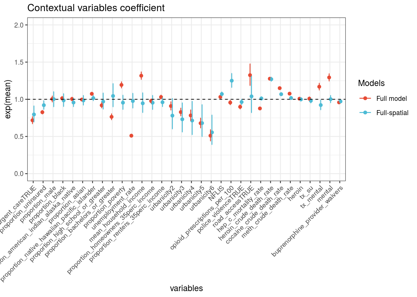
# -----------------
# Year Random Effects
# -----------------
m.N[[12]] %>% plot_random2(y_lab = "Relative Risk")
## [1] "Deprecated, update to plot_random3"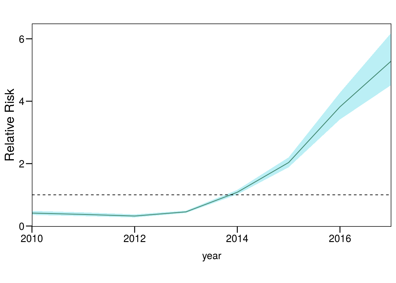
| term | mean | sd | 0.025quant | 0.5quant | 0.975quant | mode | kld |
|---|---|---|---|---|---|---|---|
| (Intercept) | -10.69 | 0.13 | -10.95 | -10.69 | -10.44 | -10.69 | 0.00 |
| urgent_careTRUE | -0.23 | 0.07 | -0.36 | -0.23 | -0.09 | -0.23 | 0.00 |
| proportion_uninsured | -0.08 | 0.03 | -0.15 | -0.08 | -0.02 | -0.08 | 0.00 |
| proportion_male | 0.00 | 0.05 | -0.11 | 0.00 | 0.10 | 0.01 | 0.00 |
| proportion_black | -0.01 | 0.04 | -0.10 | -0.01 | 0.07 | -0.02 | 0.00 |
| proportion_american_indian_alaska_native | -0.04 | 0.03 | -0.10 | -0.04 | 0.01 | -0.04 | 0.00 |
| proportion_asian | -0.01 | 0.03 | -0.08 | -0.01 | 0.05 | -0.01 | 0.00 |
| proportion_native_hawaiian_pacific_islander | 0.02 | 0.02 | -0.02 | 0.02 | 0.05 | 0.02 | 0.00 |
| proportion_high_school_or_greater | -0.03 | 0.06 | -0.14 | -0.03 | 0.08 | -0.03 | 0.00 |
| proportion_bachelors_or_greater | 0.04 | 0.08 | -0.11 | 0.04 | 0.19 | 0.04 | 0.00 |
| proportion_poverty | -0.05 | 0.05 | -0.15 | -0.05 | 0.05 | -0.05 | 0.00 |
| unemployment_rate | -0.02 | 0.05 | -0.12 | -0.02 | 0.08 | -0.02 | 0.00 |
| mean_household_income | -0.06 | 0.07 | -0.20 | -0.06 | 0.08 | -0.06 | 0.00 |
| proportion_homeowners_35perc_income | -0.05 | 0.05 | -0.15 | -0.05 | 0.05 | -0.05 | 0.00 |
| proportion_renters_35perc_income | -0.04 | 0.03 | -0.10 | -0.04 | 0.02 | -0.04 | 0.00 |
| urbanicity2 | -0.25 | 0.13 | -0.51 | -0.25 | 0.01 | -0.25 | 0.00 |
| urbanicity3 | -0.31 | 0.14 | -0.58 | -0.31 | -0.05 | -0.31 | 0.00 |
| urbanicity4 | -0.34 | 0.16 | -0.65 | -0.34 | -0.03 | -0.34 | 0.00 |
| urbanicity5 | -0.39 | 0.16 | -0.70 | -0.39 | -0.07 | -0.39 | 0.00 |
| urbanicity6 | -0.59 | 0.18 | -0.94 | -0.59 | -0.24 | -0.59 | 0.00 |
| NFLIS | 0.07 | 0.01 | 0.04 | 0.07 | 0.09 | 0.07 | 0.00 |
| opioid_prescriptions_per_100 | 0.22 | 0.04 | 0.15 | 0.22 | 0.30 | 0.22 | 0.00 |
| police_violenceTRUE | -0.04 | 0.02 | -0.08 | -0.04 | 0.00 | -0.04 | 0.00 |
| road_accessTRUE | 0.04 | 0.12 | -0.20 | 0.04 | 0.27 | 0.04 | 0.00 |
| hep_c_mortality_rate | 0.01 | 0.01 | -0.01 | 0.01 | 0.03 | 0.01 | 0.00 |
| heroin_crude_death_rate | 0.24 | 0.01 | 0.22 | 0.24 | 0.26 | 0.24 | 0.00 |
| cocaine_crude_death_rate | 0.07 | 0.01 | 0.05 | 0.07 | 0.09 | 0.07 | 0.00 |
| meth_crude_death_rate | 0.02 | 0.01 | -0.00 | 0.02 | 0.04 | 0.02 | 0.00 |
| heroin | -0.00 | 0.01 | -0.03 | -0.00 | 0.02 | -0.00 | 0.00 |
| tx_su | -0.02 | 0.02 | -0.05 | -0.02 | 0.01 | -0.02 | 0.00 |
| tx_mental | -0.08 | 0.04 | -0.15 | -0.08 | -0.01 | -0.08 | 0.00 |
| mental | 0.00 | 0.03 | -0.05 | 0.00 | 0.05 | 0.00 | 0.00 |
| buprenorphine_provider_waivers | -0.03 | 0.01 | -0.04 | -0.03 | -0.02 | -0.03 | 0.00 |
# -----------------
# Spatial Random Effect
# -----------------
m.N[[12]] %>% plot_random_map2.besag(map = usa.N, id = County.Code, col1 = NA)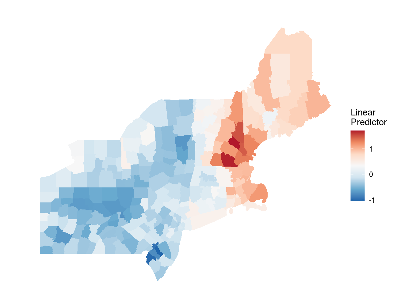
# -----------------
# RMSE
# -----------------
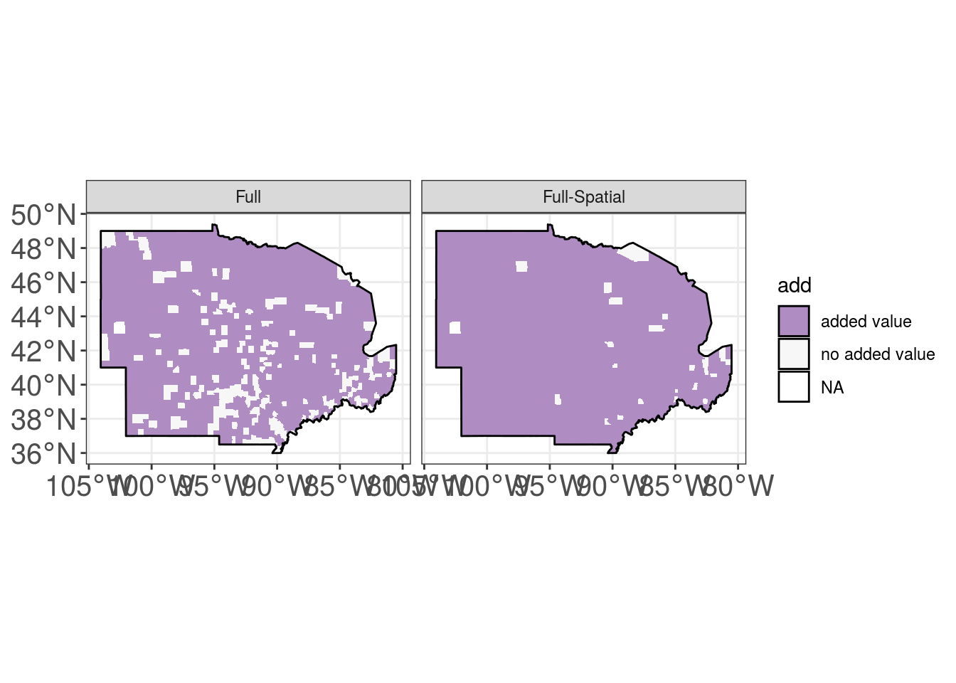
plot_rmse(dat1 = dat.N, var = synthetic_opioid_deaths, baseline = m.N[[7]],
model1 = m.N[[11]], model2 = m.N[[12]], map = usa.N, id = index,
lab1 = c("Full", "Full-Spatial"), col1 = NA)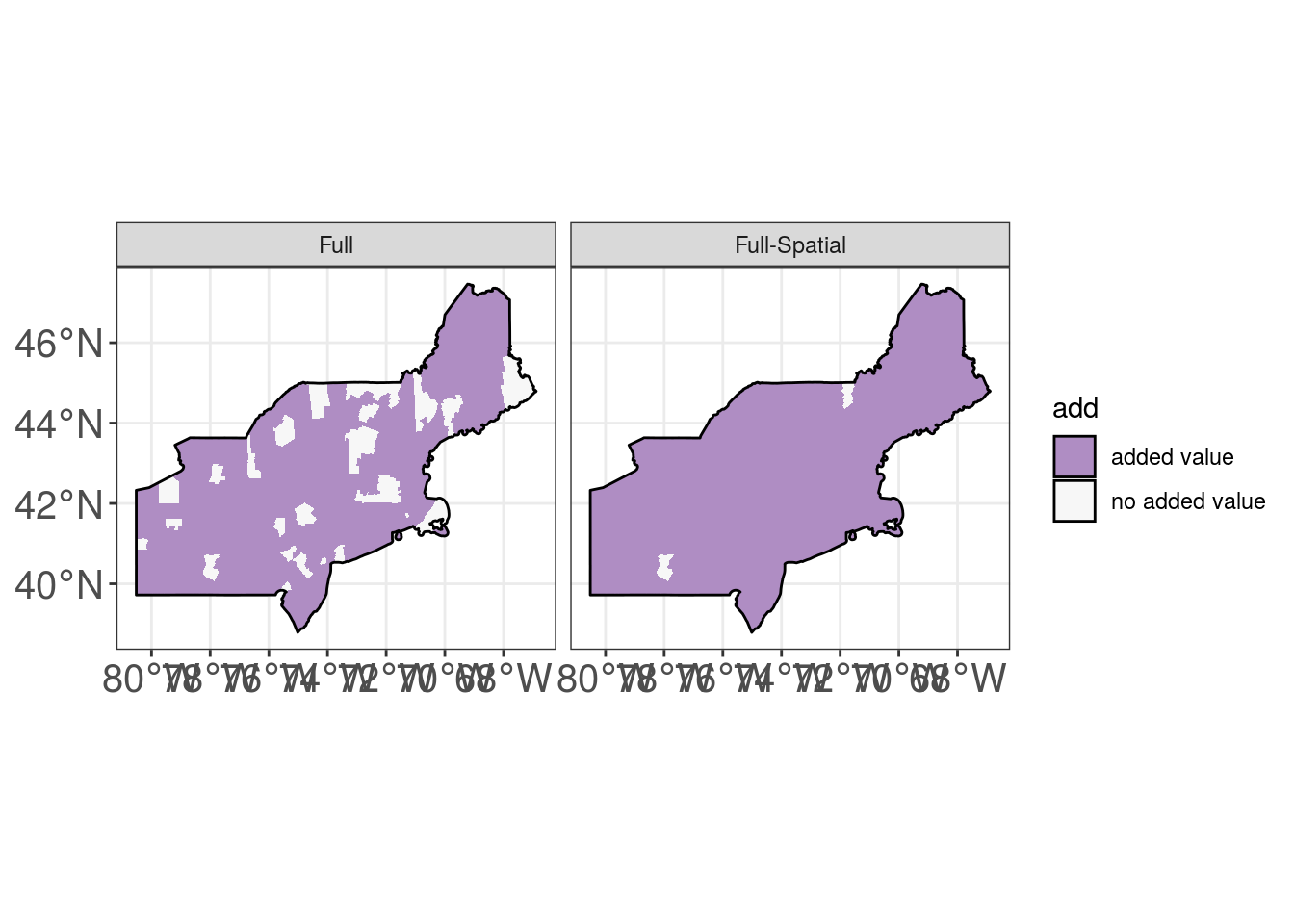
5.3.2 South
# -----------------
# Data
# -----------------
usa.S <- usa.sf %>%
  filter(loc == "S") %>%
  mutate(index = 1:n(),
         index2 = index)

nb.map.S <- poly2nb(usa.S)
#nb2INLA("map.graph.S",nb.map.S)

index.S <- usa.S %>%
  dplyr::select(County.Code, ALAND, index, index2) %>%
  st_set_geometry(NULL)

dat.S <- data %>%
  inner_join(index.S, by="County.Code") %>%
  inner_join(n.neighbors(nb.map.S), by = "index") %>%
  dplyr::select(-County.Code, -index2) %>%
  mutate(urbanicity = factor(urbanicity),
         synthetic_opioid_crude_death_rate = as.character(synthetic_opioid_crude_death_rate),
         population = as.character(population),
         synthetic_opioid_deaths = as.character(synthetic_opioid_deaths),
         year = as.character(year),
         index = as.character(index)) %>%
  mutate_if(is.numeric, scale_this) %>%
  mutate(synthetic_opioid_crude_death_rate = as.numeric(synthetic_opioid_crude_death_rate),
         population = as.numeric(population),
         synthetic_opioid_deaths = floor(as.numeric(synthetic_opioid_deaths)),
         year = as.numeric(year),
         index = as.numeric(index))

n.S<-nrow(dat.S)

# -----------------
# Formula
# -----------------

S<-c(
  # NULL
  formula = synthetic_opioid_deaths ~ 1,
  # Spatio-temporal only
  formula = synthetic_opioid_deaths ~ 1 + f(index, model = "besag", graph = "map.graph.S") + f(year, model = "rw1"),
  # Healthcare system
  formula = synthetic_opioid_deaths ~ 1 + urgent_care + proportion_uninsured + buprenorphine_provider_waivers,
  # Healthcare system spatial
  formula = synthetic_opioid_deaths ~ 1 + urgent_care + proportion_uninsured + buprenorphine_provider_waivers + f(index, model = "besag", graph = "map.graph.S") + f(year, model = "rw1"),
  #Socio-economic
  formula = synthetic_opioid_deaths ~ 1 + proportion_male + proportion_black + proportion_american_indian_alaska_native + proportion_asian + proportion_native_hawaiian_pacific_islander + proportion_high_school_or_greater + proportion_bachelors_or_greater + proportion_poverty + unemployment_rate + mean_household_income + proportion_homeowners_35perc_income + proportion_renters_35perc_income + urbanicity,
  #Socio-economic spatial
  formula = synthetic_opioid_deaths ~ 1 + proportion_male + proportion_black + proportion_american_indian_alaska_native + proportion_asian + proportion_native_hawaiian_pacific_islander + proportion_high_school_or_greater + proportion_bachelors_or_greater + proportion_poverty + unemployment_rate + mean_household_income + proportion_homeowners_35perc_income + proportion_renters_35perc_income + urbanicity + f(index, model = "besag", graph = "map.graph.S") + f(year, model = "rw1"),
  # Drug market
  formula = synthetic_opioid_deaths ~ 1 + NFLIS + opioid_prescriptions_per_100 + police_violence + road_access,
  # Drug market spatial
  formula = synthetic_opioid_deaths ~ 1 + NFLIS + opioid_prescriptions_per_100 + police_violence + road_access + f(index, model = "besag", graph = "map.graph.S") + f(year, model = "rw1"),
  # Individual susceptibility/prevalence of drug use
  formula = synthetic_opioid_deaths ~ 1 + hep_c_mortality_rate + heroin_crude_death_rate + cocaine_crude_death_rate + meth_crude_death_rate + heroin + tx_su + tx_mental + mental,
  # Individual susceptibility/prevalence of drug use spatial
  formula = synthetic_opioid_deaths ~ 1 + hep_c_mortality_rate + heroin_crude_death_rate + cocaine_crude_death_rate + meth_crude_death_rate + heroin + tx_su + tx_mental + mental + f(index, model = "besag", graph = "map.graph.S") + f(year, model = "rw1"),
  # Full model
  formula = synthetic_opioid_deaths ~ 1 + urgent_care + proportion_uninsured + proportion_male + proportion_black + proportion_american_indian_alaska_native + proportion_asian + proportion_native_hawaiian_pacific_islander + proportion_high_school_or_greater + proportion_bachelors_or_greater + proportion_poverty + unemployment_rate + mean_household_income + proportion_homeowners_35perc_income + proportion_renters_35perc_income + urbanicity + NFLIS + opioid_prescriptions_per_100 + police_violence + road_access + hep_c_mortality_rate + heroin_crude_death_rate + cocaine_crude_death_rate + meth_crude_death_rate + heroin + tx_su + tx_mental + mental + buprenorphine_provider_waivers,
  # Full-spatial model
  formula = synthetic_opioid_deaths ~ 1 + f(index, model = "besag", graph = "map.graph.S") + f(year, model = "rw1") + urgent_care + proportion_uninsured + proportion_male + proportion_black + proportion_american_indian_alaska_native + proportion_asian + proportion_native_hawaiian_pacific_islander + proportion_high_school_or_greater + proportion_bachelors_or_greater + proportion_poverty + unemployment_rate + mean_household_income + proportion_homeowners_35perc_income + proportion_renters_35perc_income + urbanicity + NFLIS + opioid_prescriptions_per_100 + police_violence + road_access + hep_c_mortality_rate + heroin_crude_death_rate + cocaine_crude_death_rate + meth_crude_death_rate + heroin + tx_su + tx_mental + mental + buprenorphine_provider_waivers)

# -----------------
# Model Estimation
# -----------------
names(S)<-c("null", "spatio-temporal", "healthcare", "healthcare spatial", "socio-economic", "socio-economic spatial",
            "drug-market", "drug-market spatial", "suscep", "suscep spatial", "full", "full-spat")

INLA:::inla.dynload.workaround()
m.S <- S %>% purrr::map(~inla.batch.safe(formula = ., dat1 = dat.S))

S.s <- m.S %>%
  purrr::map(~Rsq.batch.safe(model = ., dic.null = m.S[[1]]$dic, n = n.S)) %>%
  bind_rows(.id = "formula") %>% mutate(id = row_number())

S.s %>% plot_score()

S.s

# -----------------
# RMSE
# -----------------
library(Metrics)
dt.pred.S <- dat.S %>%
  nest() %>%
  tidyr::expand_grid(model=m.S) %>%
  mutate(id = 1:n()) %>%
  mutate(pred = purrr::map(.x = model, .f = ~.$summary.fitted.values$`0.5quant`),
         data_preds = purrr::map2(.x = data, .y = pred, .f = ~mutate(.x, pred = .y)),
         rmse = purrr::map_dbl(.x = data_preds, .f = ~rmse(actual = .$synthetic_opioid_deaths, predicted = .$pred)),
         mae = purrr::map_dbl(.x = data_preds, .f = ~mae(actual = .$synthetic_opioid_deaths, predicted = .$pred)),
         msle = purrr::map_dbl(.x = data_preds, .f = ~msle(actual = .$synthetic_opioid_deaths, predicted = .$pred)),
         mod = names(S)) %>%
dplyr::select(id, mod, rmse:msle)| id | mod | rmse | mae | msle |
|---|---|---|---|---|
| 1 | null | 10.31 | 2.23 | 0.40 |
| 2 | spatio-temporal | 2.76 | 0.65 | 0.05 |
| 3 | healthcare | 9.49 | 1.82 | 0.25 |
| 4 | healthcare spatial | 2.74 | 0.64 | 0.05 |
| 5 | socio-economic | 8.45 | 1.74 | 0.28 |
| 6 | socio-economic spatial | 2.70 | 0.64 | 0.05 |
| 7 | drug-market | 8.99 | 1.66 | 0.22 |
| 8 | drug-market spatial | 2.81 | 0.64 | 0.05 |
| 9 | suscep | 7.80 | 1.53 | 0.19 |
| 10 | suscep spatial | 2.26 | 0.58 | 0.05 |
| 11 | full | 5.73 | 1.03 | 0.11 |
| 12 | full-spat | 2.11 | 0.54 | 0.04 |
# -----------------
# Fixed Effects
# -----------------

m.S[c(11,12)] %>% plot_fixed(
  title = "Contextual variables coefficient",
  filter=10,
  lim = c("urgent_careTRUE","proportion_uninsured", "proportion_male", "proportion_black",
"proportion_american_indian_alaska_native","proportion_asian", "proportion_native_hawaiian_pacific_islander", "proportion_high_school_or_greater", "proportion_bachelors_or_greater", "proportion_poverty", "unemployment_rate", "mean_household_income", "proportion_homeowners_35perc_income", "proportion_renters_35perc_income", "urbanicity2", "urbanicity3", "urbanicity4", "urbanicity5",
"urbanicity6", "NFLIS", "opioid_prescriptions_per_100", "police_violenceTRUE", "road_accessTRUE", "hep_c_mortality_rate", "heroin_crude_death_rate", "cocaine_crude_death_rate", "meth_crude_death_rate", "heroin", "tx_su", "tx_mental", "mental", "buprenorphine_provider_waivers"),
  breaks=c("1","2"),
  lab_mod=c("Full model", "Full-spatial"), ylab = "exp(mean)", ylim = 2, b.size = 10)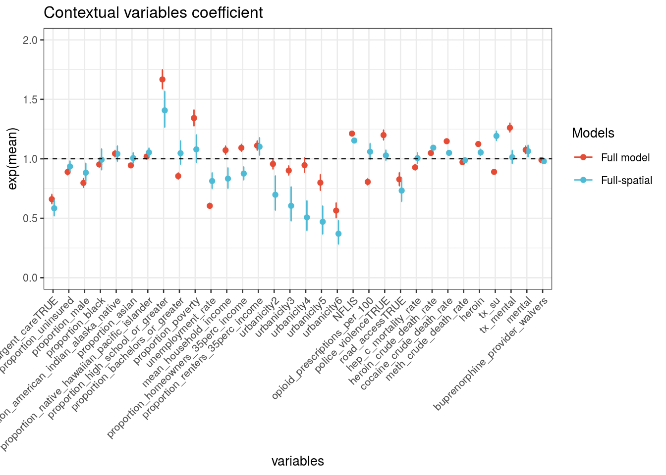
# -----------------
# Year Random Effects
# -----------------
m.S[[12]] %>% plot_random2(y_lab = "Relative Risk")
## [1] "Deprecated, update to plot_random3"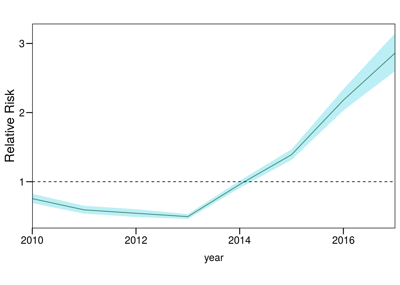
| term | mean | sd | 0.025quant | 0.5quant | 0.975quant | mode | kld |
|---|---|---|---|---|---|---|---|
| (Intercept) | -11.53 | 0.11 | -11.75 | -11.53 | -11.30 | -11.53 | 0.00 |
| urgent_careTRUE | -0.54 | 0.06 | -0.65 | -0.54 | -0.43 | -0.54 | 0.00 |
| proportion_uninsured | -0.07 | 0.02 | -0.11 | -0.07 | -0.02 | -0.07 | 0.00 |
| proportion_male | -0.12 | 0.04 | -0.21 | -0.12 | -0.04 | -0.12 | 0.00 |
| proportion_black | -0.01 | 0.04 | -0.10 | -0.01 | 0.08 | -0.01 | 0.00 |
| proportion_american_indian_alaska_native | 0.04 | 0.03 | -0.02 | 0.04 | 0.10 | 0.04 | 0.00 |
| proportion_asian | 0.01 | 0.02 | -0.04 | 0.01 | 0.05 | 0.01 | 0.00 |
| proportion_native_hawaiian_pacific_islander | 0.05 | 0.02 | 0.02 | 0.05 | 0.09 | 0.05 | 0.00 |
| proportion_high_school_or_greater | 0.34 | 0.06 | 0.23 | 0.34 | 0.45 | 0.34 | 0.00 |
| proportion_bachelors_or_greater | 0.05 | 0.05 | -0.05 | 0.05 | 0.14 | 0.05 | 0.00 |
| proportion_poverty | 0.08 | 0.05 | -0.03 | 0.08 | 0.18 | 0.08 | 0.00 |
| unemployment_rate | -0.21 | 0.04 | -0.29 | -0.21 | -0.13 | -0.21 | 0.00 |
| mean_household_income | -0.18 | 0.05 | -0.29 | -0.18 | -0.08 | -0.18 | 0.00 |
| proportion_homeowners_35perc_income | -0.13 | 0.03 | -0.19 | -0.13 | -0.07 | -0.13 | 0.00 |
| proportion_renters_35perc_income | 0.10 | 0.03 | 0.03 | 0.10 | 0.16 | 0.10 | 0.00 |
| urbanicity2 | -0.36 | 0.10 | -0.57 | -0.36 | -0.15 | -0.36 | 0.00 |
| urbanicity3 | -0.50 | 0.12 | -0.74 | -0.50 | -0.27 | -0.50 | 0.00 |
| urbanicity4 | -0.68 | 0.12 | -0.93 | -0.68 | -0.43 | -0.68 | 0.00 |
| urbanicity5 | -0.75 | 0.13 | -1.00 | -0.75 | -0.51 | -0.75 | 0.00 |
| urbanicity6 | -0.99 | 0.14 | -1.26 | -0.99 | -0.73 | -0.99 | 0.00 |
| NFLIS | 0.14 | 0.01 | 0.13 | 0.14 | 0.16 | 0.14 | 0.00 |
| opioid_prescriptions_per_100 | 0.06 | 0.03 | -0.01 | 0.06 | 0.12 | 0.06 | 0.00 |
| police_violenceTRUE | 0.03 | 0.02 | -0.01 | 0.03 | 0.07 | 0.03 | 0.00 |
| road_accessTRUE | -0.31 | 0.07 | -0.44 | -0.31 | -0.18 | -0.31 | 0.00 |
| hep_c_mortality_rate | 0.01 | 0.02 | -0.04 | 0.01 | 0.05 | 0.01 | 0.00 |
| heroin_crude_death_rate | 0.09 | 0.01 | 0.08 | 0.09 | 0.10 | 0.09 | 0.00 |
| cocaine_crude_death_rate | 0.05 | 0.01 | 0.04 | 0.05 | 0.06 | 0.05 | 0.00 |
| meth_crude_death_rate | -0.01 | 0.01 | -0.02 | -0.01 | -0.00 | -0.01 | 0.00 |
| heroin | 0.05 | 0.01 | 0.03 | 0.05 | 0.08 | 0.05 | 0.00 |
| tx_su | 0.18 | 0.02 | 0.14 | 0.18 | 0.21 | 0.18 | 0.00 |
| tx_mental | 0.01 | 0.03 | -0.04 | 0.01 | 0.07 | 0.01 | 0.00 |
| mental | 0.06 | 0.02 | 0.02 | 0.06 | 0.11 | 0.06 | 0.00 |
| buprenorphine_provider_waivers | -0.02 | 0.00 | -0.03 | -0.02 | -0.01 | -0.02 | 0.00 |
# -----------------
# Spatial Random Effect
# -----------------
m.S[[12]] %>% plot_random_map2.besag(map = usa.S, id = County.Code, col1 = NA)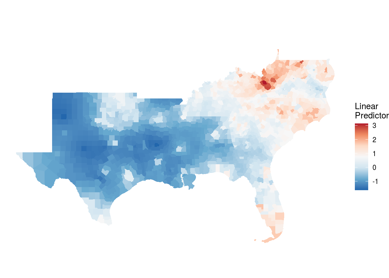
# -----------------
# RMSE
# -----------------
plot_rmse(dat1 = dat.S, var = synthetic_opioid_deaths, baseline = m.S[[7]],
          model1 = m.S[[11]], model2 = m.S[[12]], map = usa.S, id = index,
          lab1 = c("Full", "Full-Spatial"), col1 = NA)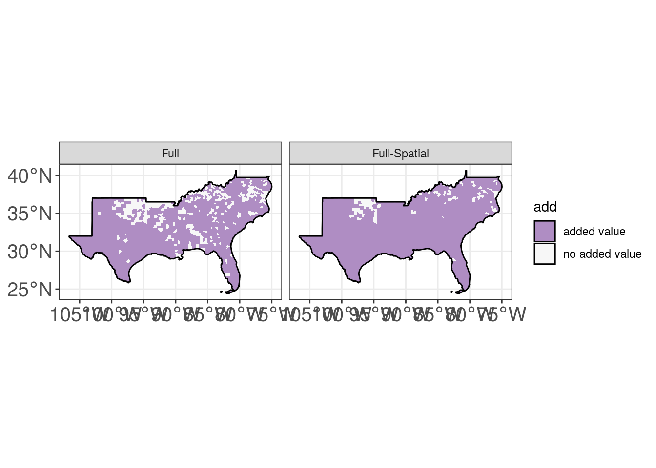
5.3.3 West
# -----------------
# Data
# -----------------
usa.W <- usa.sf %>%
  filter(loc == "W") %>%
  mutate(index = 1:n(),
         index2 = index)

nb.map.W <- poly2nb(usa.W)
#nb2INLA("map.graph.W",nb.map.W)

index.W <- usa.W %>%
  dplyr::select(County.Code, ALAND, index, index2) %>%
  st_set_geometry(NULL)

dat.W <- data %>%
  inner_join(index.W, by="County.Code") %>%
  inner_join(n.neighbors(nb.map.W), by = "index") %>%
  dplyr::select(-County.Code, -index2) %>%
  mutate(urbanicity = factor(urbanicity),
         synthetic_opioid_crude_death_rate = as.character(synthetic_opioid_crude_death_rate),
         population = as.character(population),
         synthetic_opioid_deaths = as.character(synthetic_opioid_deaths),
         year = as.character(year),
         index = as.character(index)) %>%
  mutate_if(is.numeric, scale_this) %>%
  mutate(synthetic_opioid_crude_death_rate = as.numeric(synthetic_opioid_crude_death_rate),
         population = as.numeric(population),
         synthetic_opioid_deaths = floor(as.numeric(synthetic_opioid_deaths)),
         year = as.numeric(year),
         index = as.numeric(index))

n.W<-nrow(dat.W)

# -----------------
# Formula
# -----------------

W<-c(
  # NULL
  formula = synthetic_opioid_deaths ~ 1,
  # Spatio-temporal only
  formula = synthetic_opioid_deaths ~ 1 + f(index, model = "besag", graph = "map.graph.W") + f(year, model = "rw1"),
  # Healthcare system
  formula = synthetic_opioid_deaths ~ 1 + urgent_care + proportion_uninsured + buprenorphine_provider_waivers,
  # Healthcare system spatial
  formula = synthetic_opioid_deaths ~ 1 + urgent_care + proportion_uninsured + buprenorphine_provider_waivers + f(index, model = "besag", graph = "map.graph.W") + f(year, model = "rw1"),
  #Socio-economic
  formula = synthetic_opioid_deaths ~ 1 + proportion_male + proportion_black + proportion_american_indian_alaska_native + proportion_asian + proportion_native_hawaiian_pacific_islander + proportion_high_school_or_greater + proportion_bachelors_or_greater + proportion_poverty + unemployment_rate + mean_household_income + proportion_homeowners_35perc_income + proportion_renters_35perc_income + urbanicity,
  #Socio-economic spatial
  formula = synthetic_opioid_deaths ~ 1 + proportion_male + proportion_black + proportion_american_indian_alaska_native + proportion_asian + proportion_native_hawaiian_pacific_islander + proportion_high_school_or_greater + proportion_bachelors_or_greater + proportion_poverty + unemployment_rate + mean_household_income + proportion_homeowners_35perc_income + proportion_renters_35perc_income + urbanicity + f(index, model = "besag", graph = "map.graph.W") + f(year, model = "rw1"),
  # Drug market
  formula = synthetic_opioid_deaths ~ 1 + NFLIS + opioid_prescriptions_per_100 + police_violence + road_access,
  # Drug market spatial
  formula = synthetic_opioid_deaths ~ 1 + NFLIS + opioid_prescriptions_per_100 + police_violence + road_access + f(index, model = "besag", graph = "map.graph.W") + f(year, model = "rw1"),
  # Individual susceptibility/prevalence of drug use
  formula = synthetic_opioid_deaths ~ 1 + hep_c_mortality_rate + heroin_crude_death_rate + cocaine_crude_death_rate + meth_crude_death_rate + heroin + tx_su + tx_mental + mental,
  # Individual susceptibility/prevalence of drug use spatial
  formula = synthetic_opioid_deaths ~ 1 + hep_c_mortality_rate + heroin_crude_death_rate + cocaine_crude_death_rate + meth_crude_death_rate + heroin + tx_su + tx_mental + mental + f(index, model = "besag", graph = "map.graph.W") + f(year, model = "rw1"),
  # Full model
  formula = synthetic_opioid_deaths ~ 1 + urgent_care + proportion_uninsured + proportion_male + proportion_black + proportion_american_indian_alaska_native + proportion_asian + proportion_native_hawaiian_pacific_islander + proportion_high_school_or_greater + proportion_bachelors_or_greater + proportion_poverty + unemployment_rate + mean_household_income + proportion_homeowners_35perc_income + proportion_renters_35perc_income + urbanicity + NFLIS + opioid_prescriptions_per_100 + police_violence + road_access + hep_c_mortality_rate + heroin_crude_death_rate + cocaine_crude_death_rate + meth_crude_death_rate + heroin + tx_su + tx_mental + mental + buprenorphine_provider_waivers,
  # Full-spatial model
  formula = synthetic_opioid_deaths ~ 1 + f(index, model = "besag", graph = "map.graph.W") + f(year, model = "rw1") + urgent_care + proportion_uninsured + proportion_male + proportion_black + proportion_american_indian_alaska_native + proportion_asian + proportion_native_hawaiian_pacific_islander + proportion_high_school_or_greater + proportion_bachelors_or_greater + proportion_poverty + unemployment_rate + mean_household_income + proportion_homeowners_35perc_income + proportion_renters_35perc_income + urbanicity + NFLIS + opioid_prescriptions_per_100 + police_violence + road_access + hep_c_mortality_rate + heroin_crude_death_rate + cocaine_crude_death_rate + meth_crude_death_rate + heroin + tx_su + tx_mental + mental + buprenorphine_provider_waivers)

# -----------------
# Model Estimation
# -----------------
names(W)<-c("null", "spatio-temporal", "healthcare", "healthcare spatial", "socio-economic", "socio-economic spatial",
            "drug-market", "drug-market spatial", "suscep", "suscep spatial", "full", "full-spat")

INLA:::inla.dynload.workaround()
m.W <- W %>% purrr::map(~inla.batch.safe(formula = ., dat1 = dat.W))

W.s <- m.W %>%
  purrr::map(~Rsq.batch.safe(model = ., dic.null = m.W[[1]]$dic, n = n.W)) %>%
  bind_rows(.id = "formula") %>% mutate(id = row_number())

W.s %>% plot_score()

W.s

# -----------------
# RMSE
# -----------------
library(Metrics)
dt.pred.W <- dat.W %>%
  nest() %>%
  tidyr::expand_grid(model=m.W) %>%
  mutate(id = 1:n()) %>%
  mutate(pred = purrr::map(.x = model, .f = ~.$summary.fitted.values$`0.5quant`),
         data_preds = purrr::map2(.x = data, .y = pred, .f = ~mutate(.x, pred = .y)),
         rmse = purrr::map_dbl(.x = data_preds, .f = ~rmse(actual = .$synthetic_opioid_deaths, predicted = .$pred)),
         mae = purrr::map_dbl(.x = data_preds, .f = ~mae(actual = .$synthetic_opioid_deaths, predicted = .$pred)),
         msle = purrr::map_dbl(.x = data_preds, .f = ~msle(actual = .$synthetic_opioid_deaths, predicted = .$pred)),
         mod = names(W)) %>%
dplyr::select(id, mod, rmse:msle)| id | mod | rmse | mae | msle |
|---|---|---|---|---|
| 1 | null | 5.03 | 0.99 | 0.11 |
| 2 | spatio-temporal | 2.26 | 0.44 | 0.03 |
| 3 | healthcare | 4.47 | 0.90 | 0.10 |
| 4 | healthcare spatial | 1.58 | 0.39 | 0.03 |
| 5 | socio-economic | 3.36 | 0.70 | 0.07 |
| 6 | socio-economic spatial | 2.27 | 0.44 | 0.03 |
| 7 | drug-market | 4.51 | 0.92 | 0.10 |
| 8 | drug-market spatial | 2.16 | 0.44 | 0.03 |
| 9 | suscep | 3.15 | 0.73 | 0.08 |
| 10 | suscep spatial | 1.81 | 0.40 | 0.02 |
| 11 | full | 1.97 | 0.53 | 0.05 |
| 12 | full-spat | 1.35 | 0.36 | 0.03 |
# -----------------
# Fixed Effects
# -----------------

m.W[c(11,12)] %>% plot_fixed(
  title = "Contextual variables coefficient",
  filter=10,
  lim = c("urgent_careTRUE","proportion_uninsured", "proportion_male", "proportion_black",
"proportion_american_indian_alaska_native","proportion_asian", "proportion_native_hawaiian_pacific_islander", "proportion_high_school_or_greater", "proportion_bachelors_or_greater", "proportion_poverty", "unemployment_rate", "mean_household_income", "proportion_homeowners_35perc_income", "proportion_renters_35perc_income", "urbanicity2", "urbanicity3", "urbanicity4", "urbanicity5",
"urbanicity6", "NFLIS", "opioid_prescriptions_per_100", "police_violenceTRUE", "road_accessTRUE", "hep_c_mortality_rate", "heroin_crude_death_rate", "cocaine_crude_death_rate", "meth_crude_death_rate", "heroin", "tx_su", "tx_mental", "mental", "buprenorphine_provider_waivers"),
  breaks=c("1","2"),
  lab_mod=c("Full model", "Full-spatial"), ylab = "exp(mean)", ylim = 2, b.size = 10)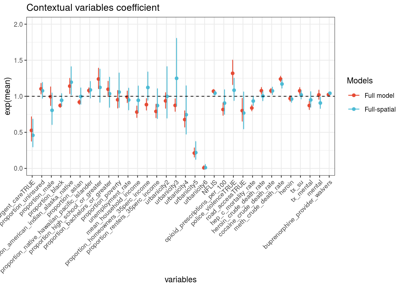
# -----------------
# Year Random Effects
# -----------------
m.W[[12]] %>% plot_random2(y_lab = "Relative Risk")
## [1] "Deprecated, update to plot_random3"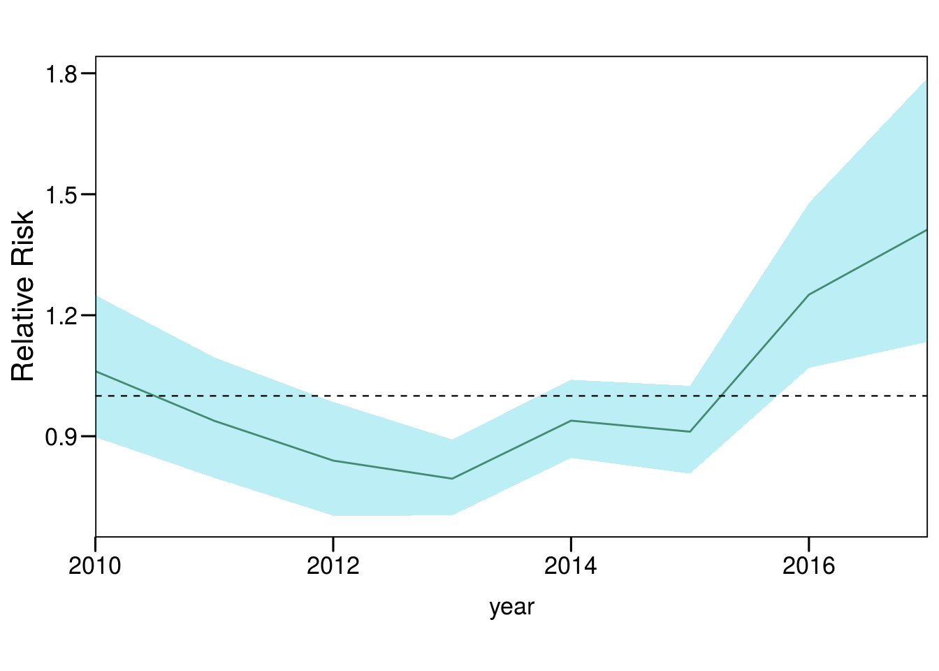
| term | mean | sd | 0.025quant | 0.5quant | 0.975quant | mode | kld |
|---|---|---|---|---|---|---|---|
| (Intercept) | -11.81 | 0.23 | -12.25 | -11.81 | -11.36 | -11.81 | 0.00 |
| urgent_careTRUE | -0.78 | 0.21 | -1.21 | -0.78 | -0.38 | -0.77 | 0.00 |
| proportion_uninsured | 0.07 | 0.05 | -0.03 | 0.07 | 0.18 | 0.07 | 0.00 |
| proportion_male | -0.22 | 0.14 | -0.50 | -0.22 | 0.04 | -0.21 | 0.00 |
| proportion_black | -0.06 | 0.05 | -0.15 | -0.06 | 0.04 | -0.06 | 0.00 |
| proportion_american_indian_alaska_native | 0.18 | 0.08 | 0.02 | 0.18 | 0.34 | 0.18 | 0.00 |
| proportion_asian | -0.00 | 0.06 | -0.12 | -0.00 | 0.11 | -0.00 | 0.00 |
| proportion_native_hawaiian_pacific_islander | 0.08 | 0.05 | -0.03 | 0.09 | 0.19 | 0.09 | 0.00 |
| proportion_high_school_or_greater | 0.12 | 0.10 | -0.09 | 0.12 | 0.32 | 0.12 | 0.00 |
| proportion_bachelors_or_greater | 0.04 | 0.10 | -0.17 | 0.04 | 0.23 | 0.04 | 0.00 |
| proportion_poverty | 0.06 | 0.12 | -0.17 | 0.06 | 0.28 | 0.06 | 0.00 |
| unemployment_rate | -0.05 | 0.08 | -0.21 | -0.05 | 0.11 | -0.05 | 0.00 |
| mean_household_income | -0.06 | 0.10 | -0.25 | -0.06 | 0.13 | -0.06 | 0.00 |
| proportion_homeowners_35perc_income | 0.12 | 0.09 | -0.06 | 0.12 | 0.29 | 0.11 | 0.00 |
| proportion_renters_35perc_income | -0.14 | 0.12 | -0.37 | -0.14 | 0.10 | -0.14 | 0.00 |
| urbanicity2 | -0.00 | 0.18 | -0.36 | -0.00 | 0.34 | 0.00 | 0.00 |
| urbanicity3 | 0.22 | 0.19 | -0.15 | 0.22 | 0.59 | 0.22 | 0.00 |
| urbanicity4 | -0.30 | 0.22 | -0.74 | -0.29 | 0.14 | -0.29 | 0.00 |
| urbanicity5 | -1.52 | 0.28 | -2.08 | -1.52 | -0.99 | -1.51 | 0.00 |
| urbanicity6 | -4.66 | 1.04 | -6.98 | -4.55 | -2.89 | -4.32 | 0.00 |
| NFLIS | 0.04 | 0.01 | 0.01 | 0.04 | 0.07 | 0.04 | 0.00 |
| opioid_prescriptions_per_100 | -0.10 | 0.10 | -0.29 | -0.10 | 0.09 | -0.10 | 0.00 |
| police_violenceTRUE | 0.08 | 0.07 | -0.06 | 0.08 | 0.23 | 0.08 | 0.00 |
| road_accessTRUE | -0.27 | 0.17 | -0.60 | -0.26 | 0.06 | -0.26 | 0.00 |
| hep_c_mortality_rate | -0.07 | 0.04 | -0.14 | -0.07 | 0.00 | -0.07 | 0.00 |
| heroin_crude_death_rate | 0.00 | 0.03 | -0.07 | 0.00 | 0.07 | 0.00 | 0.00 |
| cocaine_crude_death_rate | 0.07 | 0.03 | 0.02 | 0.07 | 0.12 | 0.07 | 0.00 |
| meth_crude_death_rate | 0.16 | 0.03 | 0.11 | 0.16 | 0.21 | 0.16 | 0.00 |
| heroin | -0.04 | 0.02 | -0.09 | -0.04 | 0.01 | -0.04 | 0.00 |
| tx_su | 0.02 | 0.03 | -0.04 | 0.02 | 0.08 | 0.02 | 0.00 |
| tx_mental | -0.05 | 0.06 | -0.17 | -0.05 | 0.06 | -0.05 | 0.00 |
| mental | -0.10 | 0.04 | -0.19 | -0.10 | -0.01 | -0.10 | 0.00 |
| buprenorphine_provider_waivers | 0.04 | 0.01 | 0.03 | 0.04 | 0.05 | 0.04 | 0.00 |
# -----------------
# Spatial Random Effect
# -----------------
m.W[[12]] %>% plot_random_map2.besag(map = usa.W, id = County.Code, col1 = NA)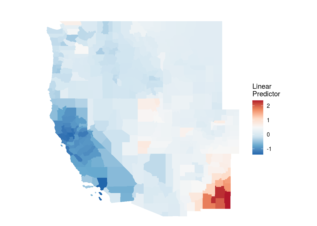
# -----------------
# RMSE
# -----------------
plot_rmse(dat1 = dat.W, var = synthetic_opioid_deaths, baseline = m.W[[7]],
          model1 = m.W[[11]], model2 = m.W[[12]], map = usa.W, id = index,
          lab1 = c("Full", "Full-Spatial"), col1 = NA)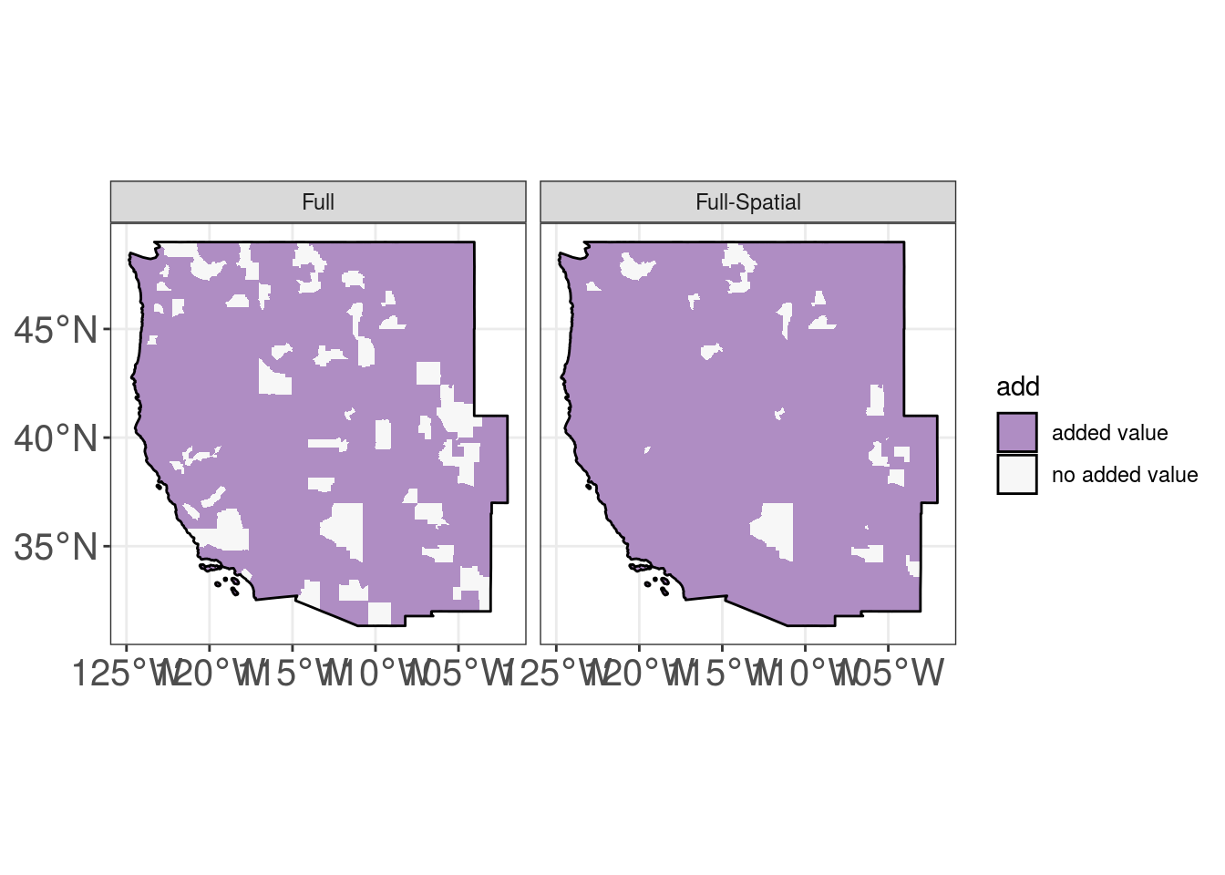
5.3.4 MidWest
# -----------------
# Data
# -----------------
usa.M <- usa.sf %>%
  filter(loc == "MW") %>%
  mutate(index = 1:n(),
         index2 = index)

nb.map.M <- poly2nb(usa.M)
#nb2INLA("map.graph.M",nb.map.M)

index.M <- usa.M %>%
  dplyr::select(County.Code, ALAND, index, index2) %>%
  st_set_geometry(NULL)

dat.M <- data %>%
  inner_join(index.M, by="County.Code") %>%
  inner_join(n.neighbors(nb.map.M), by = "index") %>%
  dplyr::select(-County.Code, -index2) %>%
  mutate(urbanicity = factor(urbanicity),
         synthetic_opioid_crude_death_rate = as.character(synthetic_opioid_crude_death_rate),
         population = as.character(population),
         synthetic_opioid_deaths = as.character(synthetic_opioid_deaths),
         year = as.character(year),
         index = as.character(index)) %>%
  mutate_if(is.numeric, scale_this) %>%
  mutate(synthetic_opioid_crude_death_rate = as.numeric(synthetic_opioid_crude_death_rate),
         population = as.numeric(population),
         synthetic_opioid_deaths = floor(as.numeric(synthetic_opioid_deaths)),
         year = as.numeric(year),
         index = as.numeric(index))

n.M<-nrow(dat.M)

# -----------------
# Formula
# -----------------

M<-c(
  # NULL
  formula = synthetic_opioid_deaths ~ 1,
  # Spatio-temporal only
  formula = synthetic_opioid_deaths ~ 1 + f(index, model = "besag", graph = "map.graph.M") + f(year, model = "rw1"),
  # Healthcare system
  formula = synthetic_opioid_deaths ~ 1 + urgent_care + proportion_uninsured + buprenorphine_provider_waivers,
  # Healthcare system spatial
  formula = synthetic_opioid_deaths ~ 1 + urgent_care + proportion_uninsured + buprenorphine_provider_waivers + f(index, model = "besag", graph = "map.graph.M") + f(year, model = "rw1"),
  #Socio-economic
  formula = synthetic_opioid_deaths ~ 1 + proportion_male + proportion_black + proportion_american_indian_alaska_native + proportion_asian + proportion_native_hawaiian_pacific_islander + proportion_high_school_or_greater + proportion_bachelors_or_greater + proportion_poverty + unemployment_rate + mean_household_income + proportion_homeowners_35perc_income + proportion_renters_35perc_income + urbanicity,
  #Socio-economic spatial
  formula = synthetic_opioid_deaths ~ 1 + proportion_male + proportion_black + proportion_american_indian_alaska_native + proportion_asian + proportion_native_hawaiian_pacific_islander + proportion_high_school_or_greater + proportion_bachelors_or_greater + proportion_poverty + unemployment_rate + mean_household_income + proportion_homeowners_35perc_income + proportion_renters_35perc_income + urbanicity + f(index, model = "besag", graph = "map.graph.M") + f(year, model = "rw1"),
  # Drug market
  formula = synthetic_opioid_deaths ~ 1 + NFLIS + opioid_prescriptions_per_100 + police_violence + road_access,
  # Drug market spatial
  formula = synthetic_opioid_deaths ~ 1 + NFLIS + opioid_prescriptions_per_100 + police_violence + road_access + f(index, model = "besag", graph = "map.graph.M") + f(year, model = "rw1"),
  # Individual susceptibility/prevalence of drug use
  formula = synthetic_opioid_deaths ~ 1 + hep_c_mortality_rate + heroin_crude_death_rate + cocaine_crude_death_rate + meth_crude_death_rate + heroin + tx_su + tx_mental + mental,
  # Individual susceptibility/prevalence of drug use spatial
  formula = synthetic_opioid_deaths ~ 1 + hep_c_mortality_rate + heroin_crude_death_rate + cocaine_crude_death_rate + meth_crude_death_rate + heroin + tx_su + tx_mental + mental + f(index, model = "besag", graph = "map.graph.M") + f(year, model = "rw1"),
  # Full model
  formula = synthetic_opioid_deaths ~ 1 + urgent_care + proportion_uninsured + proportion_male + proportion_black + proportion_american_indian_alaska_native + proportion_asian + proportion_native_hawaiian_pacific_islander + proportion_high_school_or_greater + proportion_bachelors_or_greater + proportion_poverty + unemployment_rate + mean_household_income + proportion_homeowners_35perc_income + proportion_renters_35perc_income + urbanicity + NFLIS + opioid_prescriptions_per_100 + police_violence + road_access + hep_c_mortality_rate + heroin_crude_death_rate + cocaine_crude_death_rate + meth_crude_death_rate + heroin + tx_su + tx_mental + mental + buprenorphine_provider_waivers,
  # Full-spatial model
  formula = synthetic_opioid_deaths ~ 1 + f(index, model = "besag", graph = "map.graph.M") + f(year, model = "rw1") + urgent_care + proportion_uninsured + proportion_male + proportion_black + proportion_american_indian_alaska_native + proportion_asian + proportion_native_hawaiian_pacific_islander + proportion_high_school_or_greater + proportion_bachelors_or_greater + proportion_poverty + unemployment_rate + mean_household_income + proportion_homeowners_35perc_income + proportion_renters_35perc_income + urbanicity + NFLIS + opioid_prescriptions_per_100 + police_violence + road_access + hep_c_mortality_rate + heroin_crude_death_rate + cocaine_crude_death_rate + meth_crude_death_rate + heroin + tx_su + tx_mental + mental + buprenorphine_provider_waivers)

# -----------------
# Model Estimation
# -----------------
names(M)<-c("null", "spatio-temporal", "healthcare", "healthcare spatial", "socio-economic", "socio-economic spatial",
            "drug-market", "drug-market spatial", "suscep", "suscep spatial", "full", "full-spat")

INLA:::inla.dynload.workaround()
m.M <- M %>% purrr::map(~inla.batch.safe(formula = ., dat1 = dat.M))

M.s <- m.M %>%
  purrr::map(~Rsq.batch.safe(model = ., dic.null = m.M[[1]]$dic, n = n.M)) %>%
  bind_rows(.id = "formula") %>% mutate(id = row_number())

M.s %>% plot_score()

M.s

# -----------------
# RMSE
# -----------------
library(Metrics)
dt.pred.M <- dat.M %>%
  nest() %>%
  tidyr::expand_grid(model=m.M) %>%
  mutate(id = 1:n()) %>%
  mutate(pred = purrr::map(.x = model, .f = ~.$summary.fitted.values$`0.5quant`),
         data_preds = purrr::map2(.x = data, .y = pred, .f = ~mutate(.x, pred = .y)),
         rmse = purrr::map_dbl(.x = data_preds, .f = ~rmse(actual = .$synthetic_opioid_deaths, predicted = .$pred)),
         mae = purrr::map_dbl(.x = data_preds, .f = ~mae(actual = .$synthetic_opioid_deaths, predicted = .$pred)),
         msle = purrr::map_dbl(.x = data_preds, .f = ~msle(actual = .$synthetic_opioid_deaths, predicted = .$pred)),
         mod = names(M)) %>%
dplyr::select(id, mod, rmse:msle)| id | mod | rmse | mae | msle |
|---|---|---|---|---|
| 1 | null | 15.19 | 2.58 | 0.44 |
| 2 | spatio-temporal | 3.48 | 0.60 | 0.04 |
| 3 | healthcare | 13.45 | 2.05 | 0.28 |
| 4 | healthcare spatial | 3.53 | 0.61 | 0.04 |
| 5 | socio-economic | 9.31 | 1.61 | 0.21 |
| 6 | socio-economic spatial | 3.36 | 0.59 | 0.04 |
| 7 | drug-market | 11.36 | 1.68 | 0.19 |
| 8 | drug-market spatial | 3.51 | 0.60 | 0.04 |
| 9 | suscep | 10.22 | 1.30 | 0.13 |
| 10 | suscep spatial | 3.33 | 0.56 | 0.04 |
| 11 | full | 6.28 | 0.98 | 0.08 |
| 12 | full-spat | 3.19 | 0.54 | 0.04 |
# -----------------
# Fixed Effects
# -----------------

m.M[c(11,12)] %>% plot_fixed(
  title = "Contextual variables coefficient",
  filter=10,
  lim = c("urgent_careTRUE","proportion_uninsured", "proportion_male", "proportion_black",
"proportion_american_indian_alaska_native","proportion_asian", "proportion_native_hawaiian_pacific_islander", "proportion_high_school_or_greater", "proportion_bachelors_or_greater", "proportion_poverty", "unemployment_rate", "mean_household_income", "proportion_homeowners_35perc_income", "proportion_renters_35perc_income", "urbanicity2", "urbanicity3", "urbanicity4", "urbanicity5",
"urbanicity6", "NFLIS", "opioid_prescriptions_per_100", "police_violenceTRUE", "road_accessTRUE", "hep_c_mortality_rate", "heroin_crude_death_rate", "cocaine_crude_death_rate", "meth_crude_death_rate", "heroin", "tx_su", "tx_mental", "mental", "buprenorphine_provider_waivers"),
  breaks=c("1","2"),
  lab_mod=c("Full model", "Full-spatial"), ylab = "exp(mean)", ylim = 2, b.size = 10)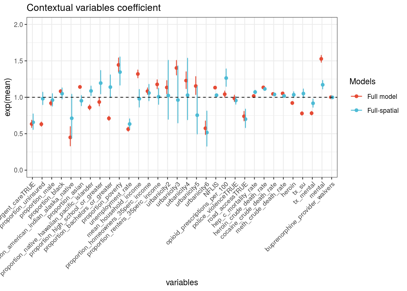
# -----------------
# Year Random Effects
# -----------------
m.M[[12]] %>% plot_random2(y_lab = "Relative Risk")
## [1] "Deprecated, update to plot_random3"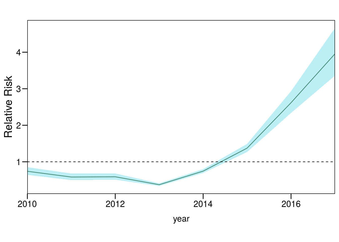
| term | mean | sd | 0.025quant | 0.5quant | 0.975quant | mode | kld |
|---|---|---|---|---|---|---|---|
| (Intercept) | -12.65 | 0.22 | -13.08 | -12.65 | -12.23 | -12.64 | 0.00 |
| urgent_careTRUE | -0.42 | 0.08 | -0.58 | -0.42 | -0.26 | -0.42 | 0.00 |
| proportion_uninsured | -0.02 | 0.04 | -0.11 | -0.02 | 0.07 | -0.02 | 0.00 |
| proportion_male | -0.04 | 0.05 | -0.13 | -0.04 | 0.05 | -0.04 | 0.00 |
| proportion_black | 0.05 | 0.04 | -0.02 | 0.05 | 0.12 | 0.05 | 0.00 |
| proportion_american_indian_alaska_native | -0.35 | 0.22 | -0.83 | -0.34 | 0.04 | -0.31 | 0.00 |
| proportion_asian | -0.05 | 0.04 | -0.12 | -0.05 | 0.03 | -0.05 | 0.00 |
| proportion_native_hawaiian_pacific_islander | 0.08 | 0.03 | 0.02 | 0.08 | 0.14 | 0.08 | 0.00 |
| proportion_high_school_or_greater | 0.18 | 0.07 | 0.04 | 0.18 | 0.31 | 0.18 | 0.00 |
| proportion_bachelors_or_greater | 0.13 | 0.07 | -0.01 | 0.13 | 0.27 | 0.13 | 0.00 |
| proportion_poverty | 0.30 | 0.07 | 0.15 | 0.30 | 0.44 | 0.30 | 0.00 |
| unemployment_rate | -0.46 | 0.06 | -0.56 | -0.46 | -0.35 | -0.46 | 0.00 |
| mean_household_income | -0.02 | 0.06 | -0.14 | -0.02 | 0.10 | -0.02 | 0.00 |
| proportion_homeowners_35perc_income | 0.06 | 0.06 | -0.05 | 0.06 | 0.16 | 0.06 | 0.00 |
| proportion_renters_35perc_income | 0.01 | 0.06 | -0.10 | 0.01 | 0.12 | 0.01 | 0.00 |
| urbanicity2 | 0.03 | 0.20 | -0.36 | 0.02 | 0.41 | 0.02 | 0.00 |
| urbanicity3 | -0.04 | 0.20 | -0.43 | -0.04 | 0.36 | -0.04 | 0.00 |
| urbanicity4 | 0.03 | 0.20 | -0.37 | 0.03 | 0.43 | 0.03 | 0.00 |
| urbanicity5 | -0.28 | 0.21 | -0.70 | -0.28 | 0.14 | -0.28 | 0.00 |
| urbanicity6 | -0.66 | 0.23 | -1.11 | -0.66 | -0.21 | -0.66 | 0.00 |
| NFLIS | 0.03 | 0.01 | 0.01 | 0.03 | 0.05 | 0.03 | 0.00 |
| opioid_prescriptions_per_100 | 0.23 | 0.05 | 0.14 | 0.23 | 0.33 | 0.23 | 0.00 |
| police_violenceTRUE | -0.04 | 0.03 | -0.10 | -0.04 | 0.01 | -0.04 | 0.00 |
| road_accessTRUE | -0.36 | 0.09 | -0.54 | -0.36 | -0.18 | -0.36 | 0.00 |
| hep_c_mortality_rate | 0.07 | 0.01 | 0.04 | 0.07 | 0.09 | 0.07 | 0.00 |
| heroin_crude_death_rate | 0.11 | 0.01 | 0.09 | 0.11 | 0.12 | 0.11 | 0.00 |
| cocaine_crude_death_rate | 0.04 | 0.01 | 0.03 | 0.04 | 0.05 | 0.04 | 0.00 |
| meth_crude_death_rate | 0.02 | 0.01 | 0.01 | 0.02 | 0.03 | 0.02 | 0.00 |
| heroin | 0.03 | 0.02 | -0.01 | 0.03 | 0.07 | 0.03 | 0.00 |
| tx_su | 0.05 | 0.03 | -0.01 | 0.05 | 0.11 | 0.05 | 0.00 |
| tx_mental | -0.09 | 0.03 | -0.15 | -0.09 | -0.02 | -0.09 | 0.00 |
| mental | 0.16 | 0.03 | 0.11 | 0.16 | 0.21 | 0.16 | 0.00 |
| buprenorphine_provider_waivers | -0.00 | 0.00 | -0.01 | -0.00 | 0.00 | -0.00 | 0.00 |
# -----------------
# Spatial Random Effect
# -----------------
m.M[[12]] %>% plot_random_map2.besag(map = usa.M, id = County.Code, col1 = NA)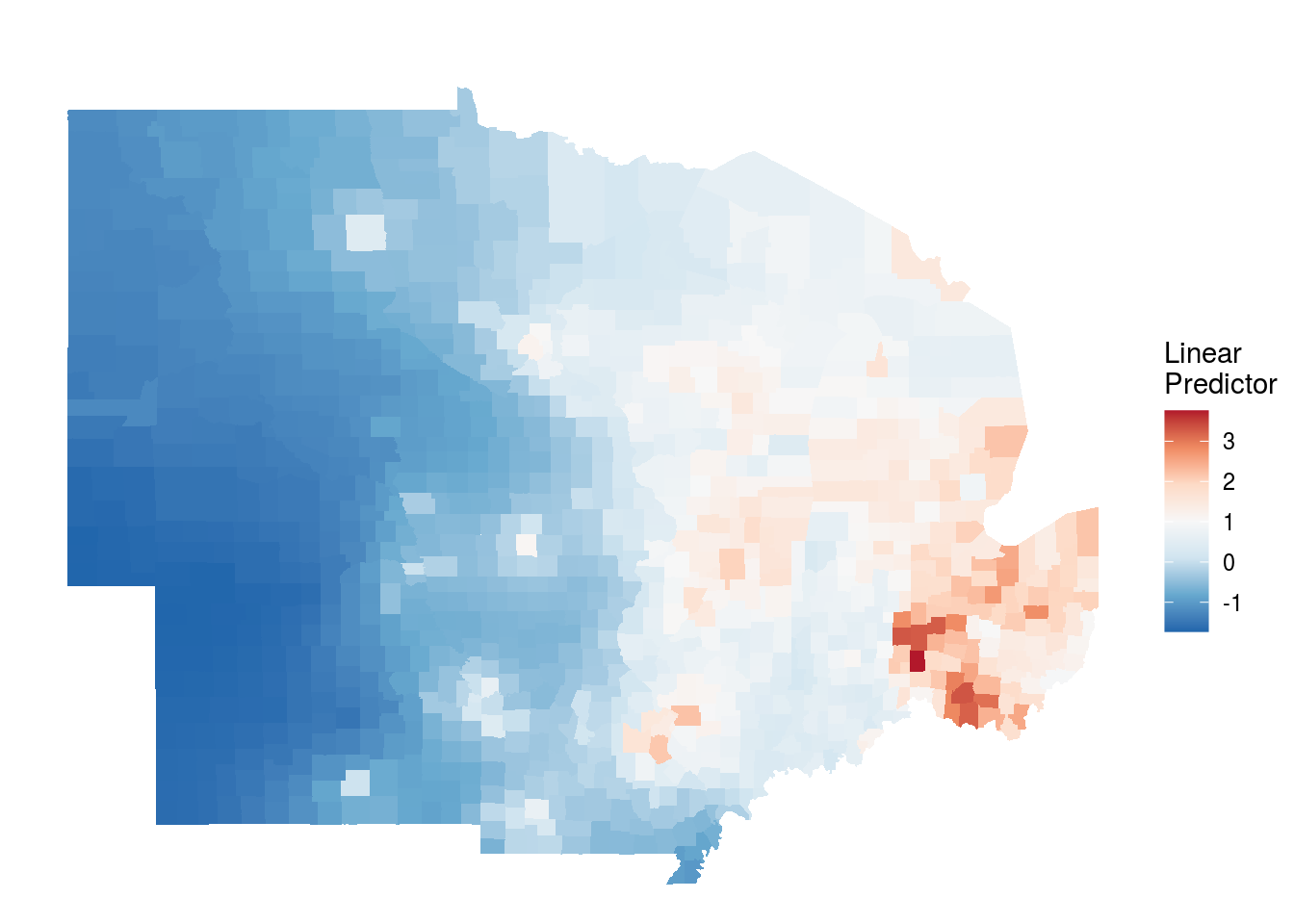
# -----------------
# RMSE
# -----------------
plot_rmse(dat1 = dat.M, var = synthetic_opioid_deaths, baseline = m.M[[7]],
          model1 = m.M[[11]], model2 = m.M[[12]], map = usa.M, id = index,
          lab1 = c("Full", "Full-Spatial"), col1 = NA)