Data
## Reading layer `tl_2017_us_county' from data source `/research-home/gcarrasco/EMMERG_MAP2/_data/GIS/tl_2017_us_county/tl_2017_us_county.shp' using driver `ESRI Shapefile'
## Simple feature collection with 3233 features and 17 fields
## geometry type:  MULTIPOLYGON
## dimension:      XY
## bbox:           xmin: -179.2311 ymin: -14.60181 xmax: 179.8597 ymax: 71.43979
## CRS:            4269
library(tidyverse); library(GGally); library(regclass); library(mctest); library(sf); library(cowplot); library(magrittr)
library(factoextra); library(olsrr)

dat.full <- data %>%
  inner_join(usa.sf %>%
               dplyr::select(County.Code, loc) %>%
               st_set_geometry(NULL) , by="County.Code")

plot.corr <- function(dat1, loc1, vars, list1=F, label1=T) {

  a <- dat1 %>%
    filter(loc==loc1) %>%
    dplyr::select(any_of(vars)) %>%
    mutate_all(as.numeric)

  abv <- abbreviate(colnames(a), 5)

  b <- a%>%
    set_colnames(abv) %>%
    GGally::ggcorr(label = label1, label_round = 4, hjust=1) +
    ggtitle(paste0("Area: ", loc1, "; n=", nrow(a)))

  if (isTRUE(list1)) {print(abv)}

  return(b)
}

summ.pca <- function(res.pca){
  # Eigenvalues
  eig <- (res.pca$sdev)^2
  # Diff Eigenvalues
  diff <- -diff(eig)
  diff[length(eig)]<-NA
  # Variances in proportion
  variance <- eig/sum(eig)
  # Cumulative variances
  cumvar <- cumsum(variance)

  eig.summ <- data.frame(eig = eig, diff= diff, variance = variance,cumvariance = cumvar)

  return(eig.summ)

}
Healthcare system
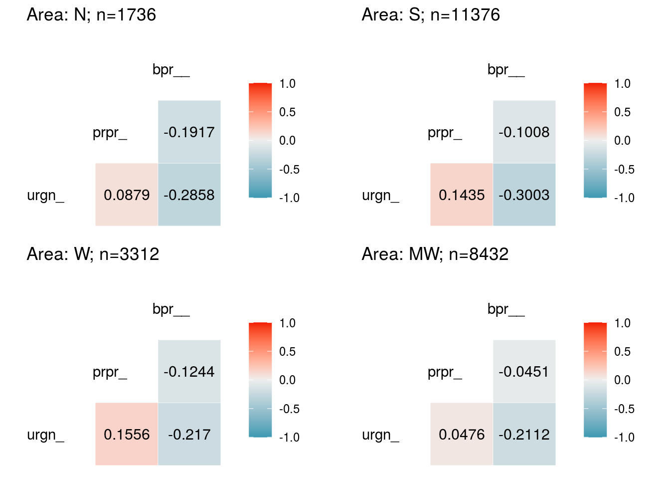
# Correlation
vars_hcs <- c("urgent_care", "proportion_uninsured", "buprenorphine_provider_waivers")

hcs_a <- plot.corr(dat.full, loc1 = "N", vars = vars_hcs, list1 = T)
##                    urgent_care           proportion_uninsured
##                        "urgn_"                        "prpr_"
## buprenorphine_provider_waivers
##                        "bpr__"
hcs_b <- plot.corr(dat.full, loc1 = "S", vars = vars_hcs)
hcs_c <- plot.corr(dat.full, loc1 = "W", vars = vars_hcs)
hcs_d <- plot.corr(dat.full, loc1 = "MW", vars = vars_hcs)

plot_grid(hcs_a, hcs_b, hcs_c, hcs_d)
# PCA
res.pca_hcs <- dat.full %>%
  dplyr::select(any_of(vars_hcs)) %>%
  mutate_all(as.numeric) %>%
  filter(complete.cases(.)) %>%
  princomp(cor = TRUE, scores = TRUE)

fviz_eig(res.pca_hcs)
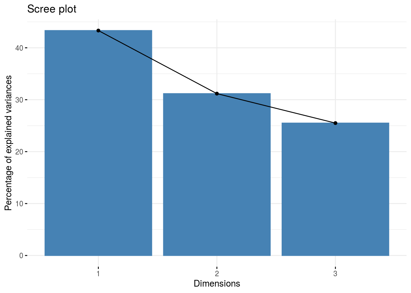
(summ.pca_hcs <- summ.pca(res.pca_hcs))
##              eig      diff  variance cumvariance
## Comp.1 1.2997242 0.3644972 0.4332414   0.4332414
## Comp.2 0.9352270 0.1701781 0.3117423   0.7449837
## Comp.3 0.7650489        NA 0.2550163   1.0000000
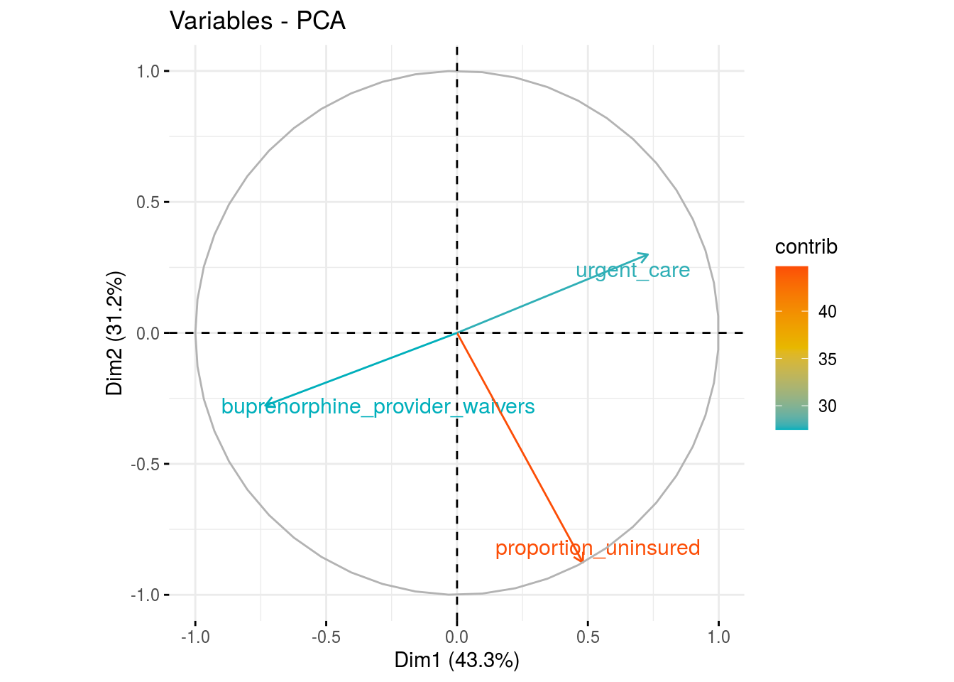
fviz_pca_var(res.pca_hcs,
             col.var = "contrib",
             gradient.cols = c("#00AFBB", "#E7B800", "#FC4E07"),
             repel = TRUE)
Socio-economic
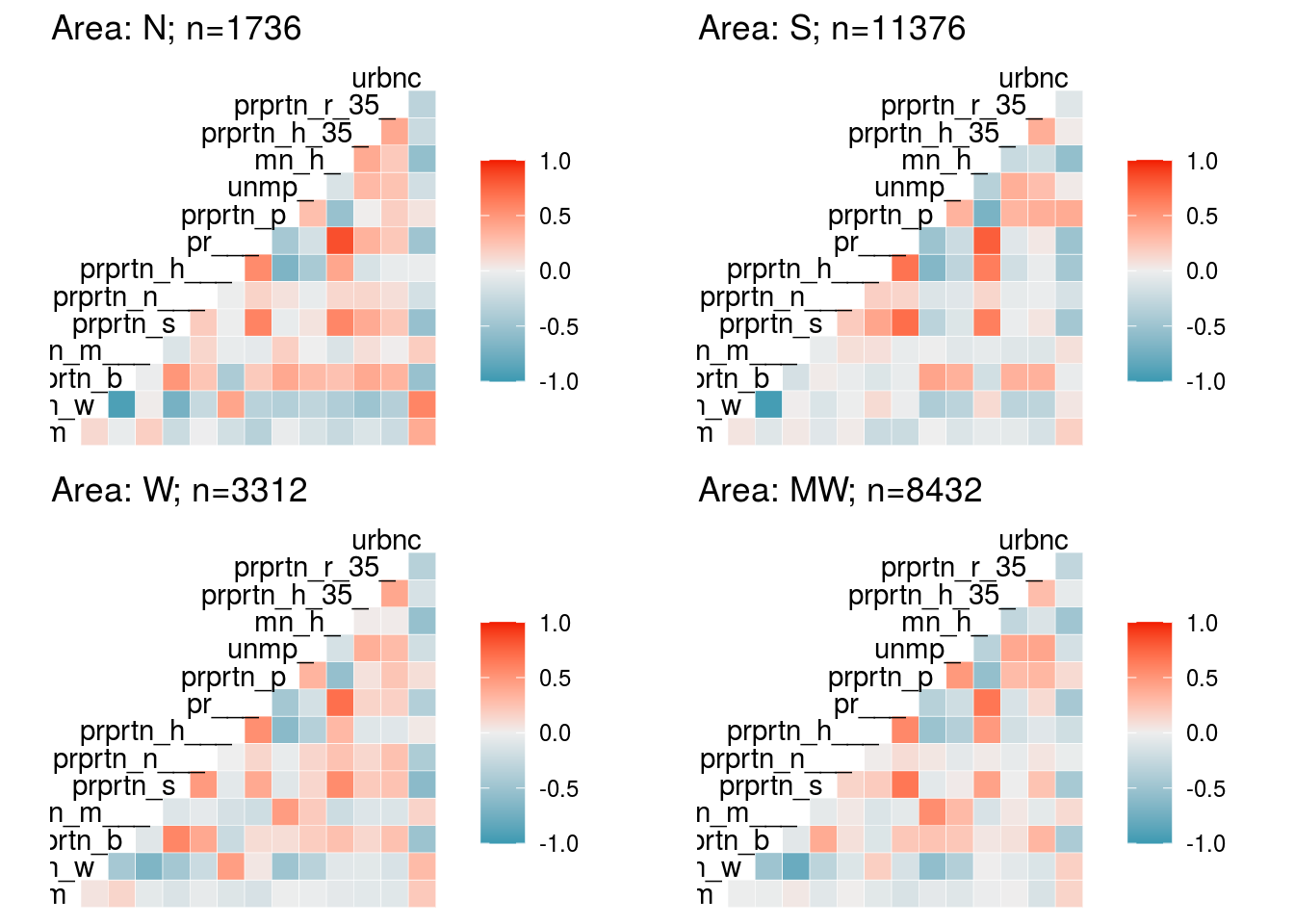
# Correlation
vars_ses <- c("proportion_male", "proportion_white", "proportion_black", "proportion_american_indian_alaska_native", "proportion_asian",
"proportion_native_hawaiian_pacific_islander", "proportion_high_school_or_greater", "proportion_bachelors_or_greater",
"proportion_poverty", "unemployment_rate", "mean_household_income", "proportion_homeowners_35perc_income",
"proportion_renters_35perc_income", "urbanicity")
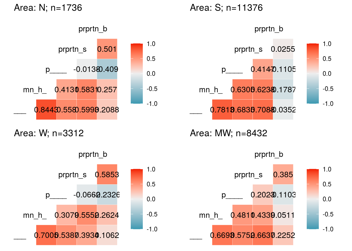
ses_a <- plot.corr(dat.full, loc1 = "N", vars = vars_ses, label1 = F, list1 = T)
##                             proportion_male
##                                  "prprtn_m"
##                            proportion_white
##                                  "prprtn_w"
##                            proportion_black
##                                  "prprtn_b"
##    proportion_american_indian_alaska_native
##                               "prprtn_m___"
##                            proportion_asian
##                                  "prprtn_s"
## proportion_native_hawaiian_pacific_islander
##                               "prprtn_n___"
##           proportion_high_school_or_greater
##                               "prprtn_h___"
##             proportion_bachelors_or_greater
##                                     "pr___"
##                          proportion_poverty
##                                  "prprtn_p"
##                           unemployment_rate
##                                     "unmp_"
##                       mean_household_income
##                                     "mn_h_"
##         proportion_homeowners_35perc_income
##                              "prprtn_h_35_"
##            proportion_renters_35perc_income
##                              "prprtn_r_35_"
##                                  urbanicity
##                                     "urbnc"
ses_b <- plot.corr(dat.full, loc1 = "S", vars = vars_ses, label1 = F)
ses_c <- plot.corr(dat.full, loc1 = "W", vars = vars_ses, label1 = F)
ses_d <- plot.corr(dat.full, loc1 = "MW", vars = vars_ses, label1 = F)

plot_grid(ses_a, ses_b, ses_c, ses_d)
vars_ses1 <- c("proportion_bachelors_or_greater", "mean_household_income", "proportion_high_school_or_greater", "proportion_asian",
               "proportion_black")

ses1_a <- plot.corr(dat.full, loc1 = "N", vars = vars_ses1, label1 = T, list1 = T)
##   proportion_bachelors_or_greater             mean_household_income
##                           "pr___"                           "mn_h_"
## proportion_high_school_or_greater                  proportion_asian
##                           "p____"                        "prprtn_s"
##                  proportion_black
##                        "prprtn_b"
ses1_b <- plot.corr(dat.full, loc1 = "S", vars = vars_ses1, label1 = T)
ses1_c <- plot.corr(dat.full, loc1 = "W", vars = vars_ses1, label1 = T)
ses1_d <- plot.corr(dat.full, loc1 = "MW", vars = vars_ses1, label1 = T)

plot_grid(ses1_a, ses1_b, ses1_c, ses1_d)
# PCA
res.pca_ses <- dat.full %>%
  dplyr::select(any_of(vars_ses)) %>%
  mutate_all(as.numeric) %>%
  filter(complete.cases(.)) %>%
  princomp(cor = TRUE, scores = TRUE)

fviz_eig(res.pca_ses)
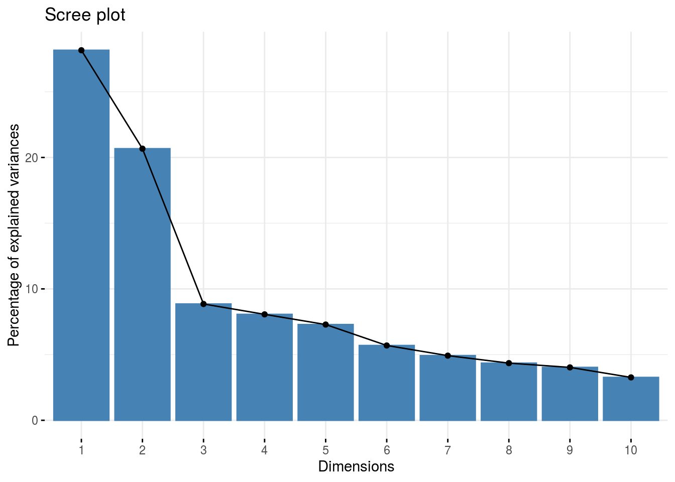
(summ.pca_ses <- summ.pca(res.pca_ses))
##                eig       diff    variance cumvariance
## Comp.1  3.94225819 1.04880194 0.281589871   0.2815899
## Comp.2  2.89345625 1.65451033 0.206675446   0.4882653
## Comp.3  1.23894592 0.11044029 0.088496137   0.5767615
## Comp.4  1.12850562 0.10852003 0.080607544   0.6573690
## Comp.5  1.01998559 0.22319541 0.072856114   0.7302251
## Comp.6  0.79679018 0.10815890 0.056913584   0.7871387
## Comp.7  0.68863127 0.07971270 0.049187948   0.8363266
## Comp.8  0.60891857 0.04550467 0.043494184   0.8798208
## Comp.9  0.56341390 0.10666293 0.040243850   0.9200647
## Comp.10 0.45675097 0.17765147 0.032625069   0.9526897
## Comp.11 0.27909950 0.04873961 0.019935679   0.9726254
## Comp.12 0.23035989 0.10025375 0.016454278   0.9890797
## Comp.13 0.13010614 0.10732815 0.009293296   0.9983730
## Comp.14 0.02277799         NA 0.001627000   1.0000000
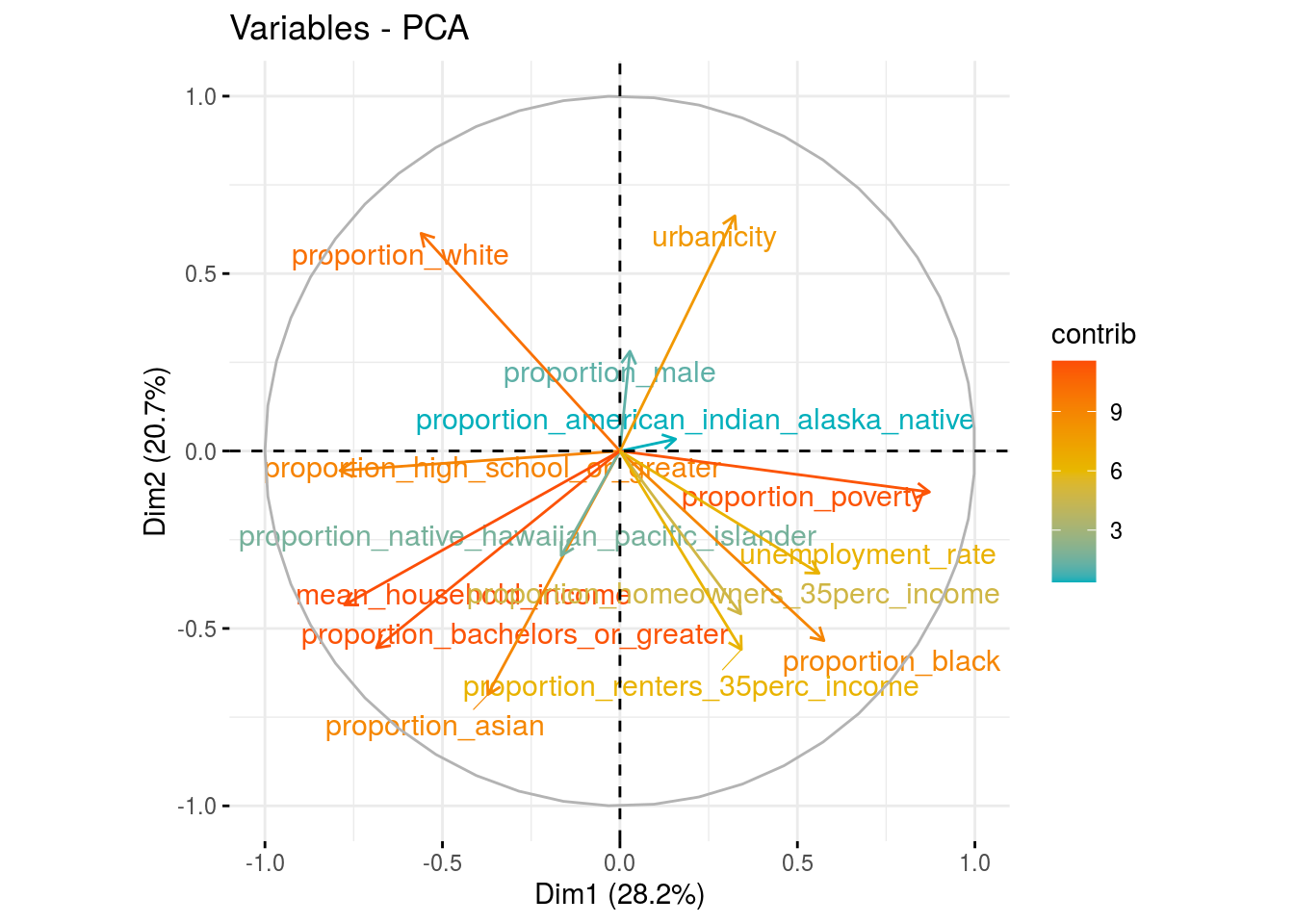
fviz_pca_var(res.pca_ses,
             col.var = "contrib",
             gradient.cols = c("#00AFBB", "#E7B800", "#FC4E07"),
             repel = TRUE)
# VIF & TOL
model_ses<-lm(synthetic_opioid_crude_death_rate ~ proportion_male + proportion_white + proportion_black +
                proportion_american_indian_alaska_native + proportion_asian + proportion_native_hawaiian_pacific_islander +
                proportion_high_school_or_greater + proportion_bachelors_or_greater + proportion_poverty + unemployment_rate +
                mean_household_income + proportion_homeowners_35perc_income + proportion_renters_35perc_income + urbanicity,
              data = dat.full, na.action=na.exclude)

summary(model_ses)
##
## Call:
## lm(formula = synthetic_opioid_crude_death_rate ~ proportion_male +
##     proportion_white + proportion_black + proportion_american_indian_alaska_native +
##     proportion_asian + proportion_native_hawaiian_pacific_islander +
##     proportion_high_school_or_greater + proportion_bachelors_or_greater +
##     proportion_poverty + unemployment_rate + mean_household_income +
##     proportion_homeowners_35perc_income + proportion_renters_35perc_income +
##     urbanicity, data = dat.full, na.action = na.exclude)
##
## Residuals:
##     Min      1Q  Median      3Q     Max
##  -5.239  -1.576  -0.743   0.326 119.722
##
## Coefficients:
##                                               Estimate Std. Error t value
## (Intercept)                                 -9.370e+00  1.086e+00  -8.626
## proportion_male                             -6.148e-02  1.136e-02  -5.413
## proportion_white                             1.051e-01  7.268e-03  14.463
## proportion_black                             9.260e-02  7.264e-03  12.748
## proportion_american_indian_alaska_native     6.601e-02  7.651e-03   8.628
## proportion_asian                             6.005e-02  1.643e-02   3.655
## proportion_native_hawaiian_pacific_islander -4.896e-01  1.128e-01  -4.342
## proportion_high_school_or_greater            2.977e-02  6.370e-03   4.673
## proportion_bachelors_or_greater             -2.397e-02  5.318e-03  -4.508
## proportion_poverty                           1.544e-01  8.820e-03  17.502
## unemployment_rate                           -2.234e-01  9.794e-03 -22.805
## mean_household_income                        4.344e-05  3.424e-06  12.685
## proportion_homeowners_35perc_income         -2.464e-02  4.084e-03  -6.032
## proportion_renters_35perc_income             3.735e-02  3.467e-03  10.772
## urbanicity                                  -3.302e-01  2.166e-02 -15.249
##                                             Pr(>|t|)
## (Intercept)                                  < 2e-16 ***
## proportion_male                             6.26e-08 ***
## proportion_white                             < 2e-16 ***
## proportion_black                             < 2e-16 ***
## proportion_american_indian_alaska_native     < 2e-16 ***
## proportion_asian                            0.000257 ***
## proportion_native_hawaiian_pacific_islander 1.42e-05 ***
## proportion_high_school_or_greater           2.98e-06 ***
## proportion_bachelors_or_greater             6.58e-06 ***
## proportion_poverty                           < 2e-16 ***
## unemployment_rate                            < 2e-16 ***
## mean_household_income                        < 2e-16 ***
## proportion_homeowners_35perc_income         1.64e-09 ***
## proportion_renters_35perc_income             < 2e-16 ***
## urbanicity                                   < 2e-16 ***
## ---
## Signif. codes:  0 '***' 0.001 '**' 0.01 '*' 0.05 '.' 0.1 ' ' 1
##
## Residual standard error: 3.916 on 24841 degrees of freedom
## Multiple R-squared:  0.07712,	Adjusted R-squared:  0.0766
## F-statistic: 148.3 on 14 and 24841 DF,  p-value: < 2.2e-16
##                                      Variables  Tolerance       VIF
## 1                              proportion_male 0.88558207  1.129201
## 2                             proportion_white 0.04567660 21.893048
## 3                             proportion_black 0.05394956 18.535833
## 4     proportion_american_indian_alaska_native 0.22394963  4.465290
## 5                             proportion_asian 0.38359167  2.606939
## 6  proportion_native_hawaiian_pacific_islander 0.84200651  1.187639
## 7            proportion_high_school_or_greater 0.31584003  3.166160
## 8              proportion_bachelors_or_greater 0.27243079  3.670657
## 9                           proportion_poverty 0.25111251  3.982279
## 10                           unemployment_rate 0.64094685  1.560192
## 11                       mean_household_income 0.24054204  4.157277
## 12         proportion_homeowners_35perc_income 0.73401336  1.362373
## 13            proportion_renters_35perc_income 0.60883323  1.642486
## 14                                  urbanicity 0.57493601  1.739324
# proportion_white/proportion_black VIF>10 and TOL<0.1

model_ses1<-lm(synthetic_opioid_crude_death_rate ~ proportion_male + proportion_black +
                proportion_american_indian_alaska_native + proportion_asian + proportion_native_hawaiian_pacific_islander +
                proportion_high_school_or_greater + proportion_bachelors_or_greater + proportion_poverty + unemployment_rate +
                mean_household_income + proportion_homeowners_35perc_income + proportion_renters_35perc_income + urbanicity,
              data = dat.full, na.action=na.exclude)

summary(model_ses1)
##
## Call:
## lm(formula = synthetic_opioid_crude_death_rate ~ proportion_male +
##     proportion_black + proportion_american_indian_alaska_native +
##     proportion_asian + proportion_native_hawaiian_pacific_islander +
##     proportion_high_school_or_greater + proportion_bachelors_or_greater +
##     proportion_poverty + unemployment_rate + mean_household_income +
##     proportion_homeowners_35perc_income + proportion_renters_35perc_income +
##     urbanicity, data = dat.full, na.action = na.exclude)
##
## Residuals:
##     Min      1Q  Median      3Q     Max
##  -4.836  -1.590  -0.753   0.323 119.857
##
## Coefficients:
##                                               Estimate Std. Error t value
## (Intercept)                                 -3.371e-01  8.925e-01  -0.378
## proportion_male                             -7.116e-02  1.139e-02  -6.250
## proportion_black                            -7.875e-03  2.132e-03  -3.693
## proportion_american_indian_alaska_native    -2.672e-02  4.192e-03  -6.374
## proportion_asian                            -5.397e-02  1.447e-02  -3.729
## proportion_native_hawaiian_pacific_islander -6.357e-01  1.128e-01  -5.637
## proportion_high_school_or_greater            5.796e-02  6.090e-03   9.517
## proportion_bachelors_or_greater             -2.752e-02  5.334e-03  -5.159
## proportion_poverty                           1.481e-01  8.846e-03  16.737
## unemployment_rate                           -2.247e-01  9.835e-03 -22.849
## mean_household_income                        3.698e-05  3.409e-06  10.846
## proportion_homeowners_35perc_income         -2.808e-02  4.095e-03  -6.859
## proportion_renters_35perc_income             4.041e-02  3.475e-03  11.626
## urbanicity                                  -3.290e-01  2.175e-02 -15.129
##                                             Pr(>|t|)
## (Intercept)                                 0.705605
## proportion_male                             4.17e-10 ***
## proportion_black                            0.000222 ***
## proportion_american_indian_alaska_native    1.87e-10 ***
## proportion_asian                            0.000193 ***
## proportion_native_hawaiian_pacific_islander 1.75e-08 ***
## proportion_high_school_or_greater            < 2e-16 ***
## proportion_bachelors_or_greater             2.50e-07 ***
## proportion_poverty                           < 2e-16 ***
## unemployment_rate                            < 2e-16 ***
## mean_household_income                        < 2e-16 ***
## proportion_homeowners_35perc_income         7.10e-12 ***
## proportion_renters_35perc_income             < 2e-16 ***
## urbanicity                                   < 2e-16 ***
## ---
## Signif. codes:  0 '***' 0.001 '**' 0.01 '*' 0.05 '.' 0.1 ' ' 1
##
## Residual standard error: 3.932 on 24842 degrees of freedom
## Multiple R-squared:  0.06935,	Adjusted R-squared:  0.06886
## F-statistic: 142.4 on 13 and 24842 DF,  p-value: < 2.2e-16
##                                      Variables Tolerance      VIF
## 1                              proportion_male 0.8886685 1.125279
## 2                             proportion_black 0.6313744 1.583846
## 3     proportion_american_indian_alaska_native 0.7521561 1.329511
## 4                             proportion_asian 0.4983396 2.006664
## 5  proportion_native_hawaiian_pacific_islander 0.8488200 1.178106
## 6            proportion_high_school_or_greater 0.3484586 2.869781
## 7              proportion_bachelors_or_greater 0.2730117 3.662846
## 8                           proportion_poverty 0.2517280 3.972541
## 9                            unemployment_rate 0.6410056 1.560049
## 10                       mean_household_income 0.2447074 4.086512
## 11         proportion_homeowners_35perc_income 0.7365210 1.357734
## 12            proportion_renters_35perc_income 0.6111010 1.636391
## 13                                  urbanicity 0.5749449 1.739297
Drug market
# Correlation
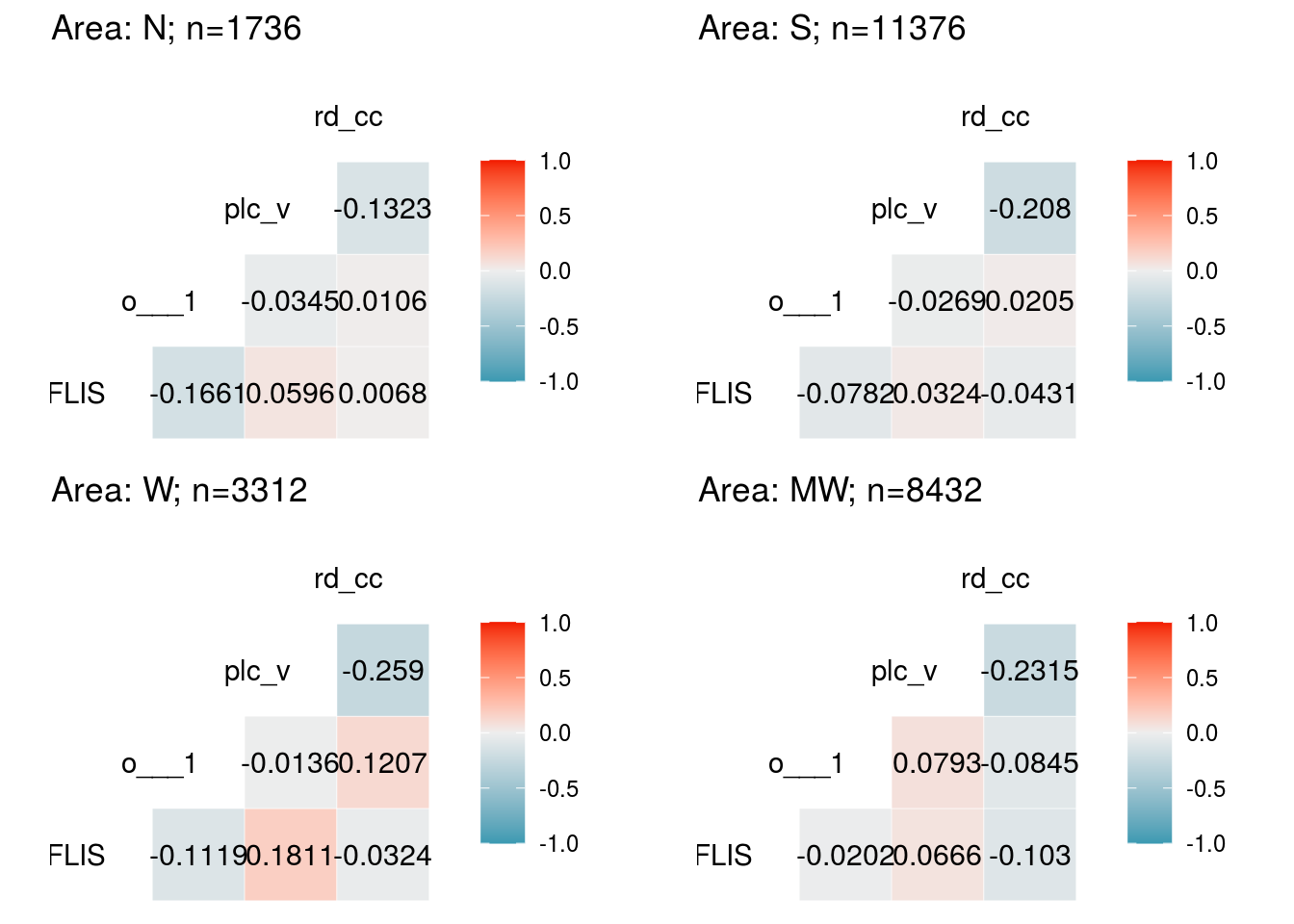
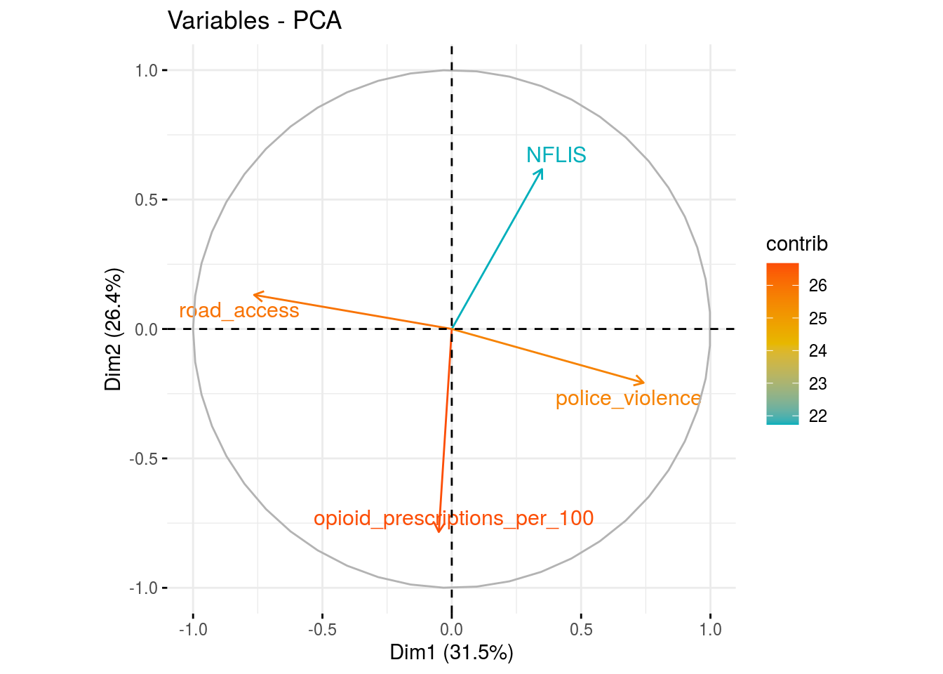
vars_dm <- c("NFLIS", "opioid_prescriptions_per_100", "police_violence", "road_access")
dm_a <- plot.corr(dat.full, loc1 = "N", vars = vars_dm, label1 = T, list1 = T)
##                        NFLIS opioid_prescriptions_per_100
##                      "NFLIS"                      "o___1"
##              police_violence                  road_access
##                      "plc_v"                      "rd_cc"
dm_b <- plot.corr(dat.full, loc1 = "S", vars = vars_dm, label1 = T)
dm_c <- plot.corr(dat.full, loc1 = "W", vars = vars_dm, label1 = T)
dm_d <- plot.corr(dat.full, loc1 = "MW", vars = vars_dm, label1 = T)

plot_grid(dm_a, dm_b, dm_c, dm_d)
# PCA
res.pca_dm <- dat.full %>%
  dplyr::select(any_of(vars_dm)) %>%
  mutate_all(as.numeric) %>%
  filter(complete.cases(.)) %>%
  princomp(cor = TRUE, scores = TRUE)

fviz_eig(res.pca_dm)
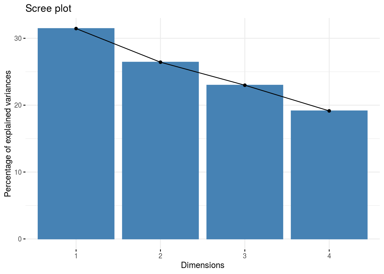
(summ.pca_dm <- summ.pca(res.pca_dm))
##              eig      diff  variance cumvariance
## Comp.1 1.2580763 0.2011132 0.3145191   0.3145191
## Comp.2 1.0569631 0.1376957 0.2642408   0.5787599
## Comp.3 0.9192674 0.1535743 0.2298169   0.8085767
## Comp.4 0.7656931        NA 0.1914233   1.0000000
fviz_pca_var(res.pca_dm,
             col.var = "contrib",
             gradient.cols = c("#00AFBB", "#E7B800", "#FC4E07"),
             repel = TRUE)
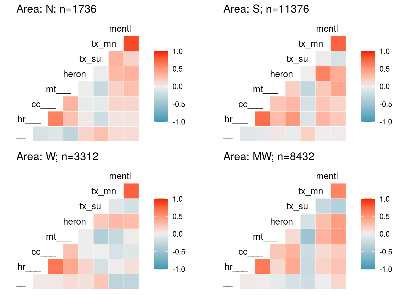
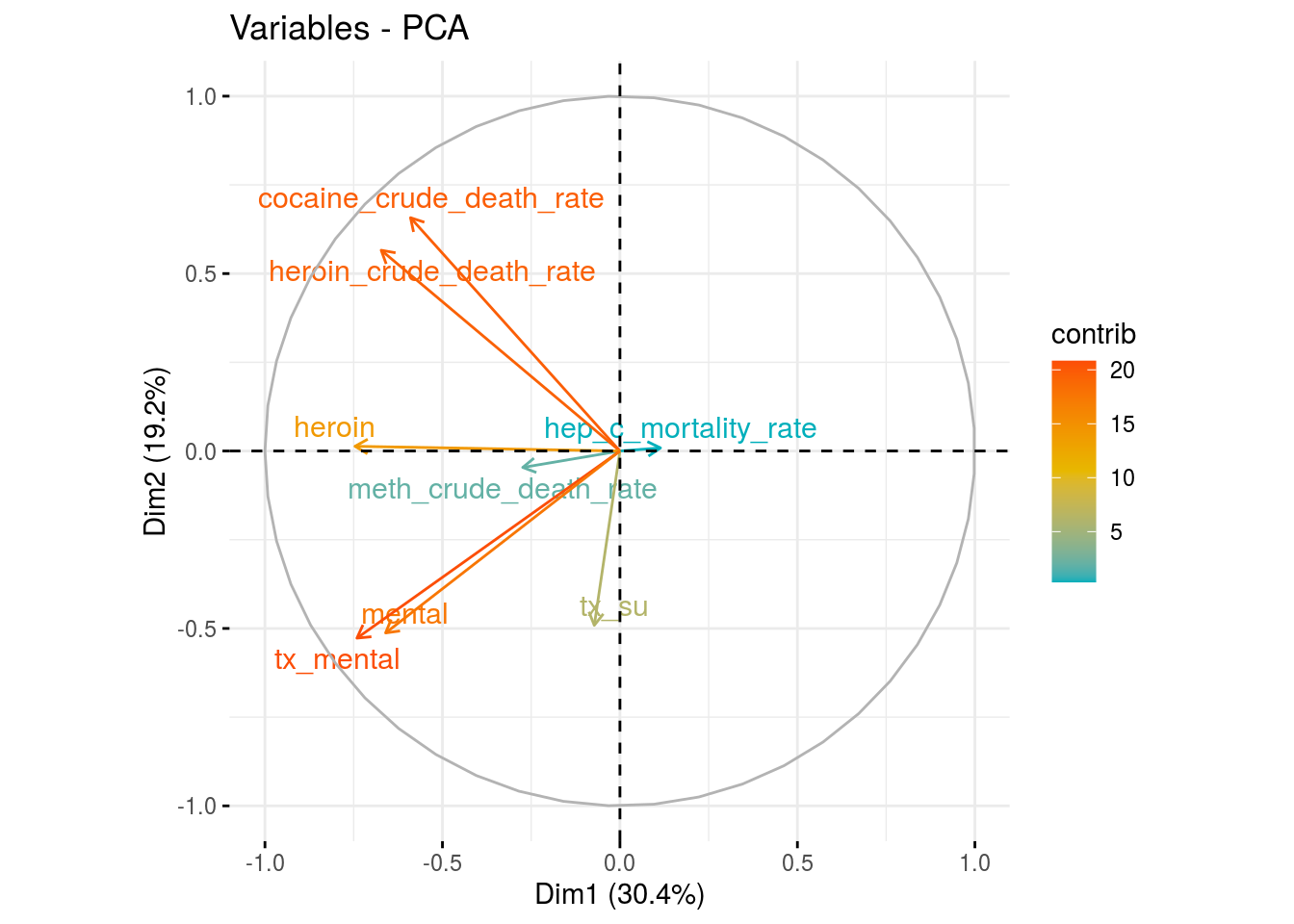
Individual susceptibility/prevalence of drug use
# Correlation
vars_sus <- c("hep_c_mortality_rate", "heroin_crude_death_rate", "cocaine_crude_death_rate", "meth_crude_death_rate", "heroin", "tx_su",
              "tx_mental", "mental")

sus_a <- plot.corr(dat.full, loc1 = "N", vars = vars_sus, label1 = F, list1 = T)
##     hep_c_mortality_rate  heroin_crude_death_rate cocaine_crude_death_rate
##                  "hp___"                  "hr___"                  "cc___"
##    meth_crude_death_rate                   heroin                    tx_su
##                  "mt___"                  "heron"                  "tx_su"
##                tx_mental                   mental
##                  "tx_mn"                  "mentl"
sus_b <- plot.corr(dat.full, loc1 = "S", vars = vars_sus, label1 = F)
sus_c <- plot.corr(dat.full, loc1 = "W", vars = vars_sus, label1 = F)
sus_d <- plot.corr(dat.full, loc1 = "MW", vars = vars_sus, label1 = F)

plot_grid(sus_a, sus_b, sus_c, sus_d)
# PCA
res.pca_sus <- dat.full %>%
  dplyr::select(any_of(vars_sus)) %>%
  mutate_all(as.numeric) %>%
  filter(complete.cases(.)) %>%
  princomp(cor = TRUE, scores = TRUE)

fviz_eig(res.pca_sus)
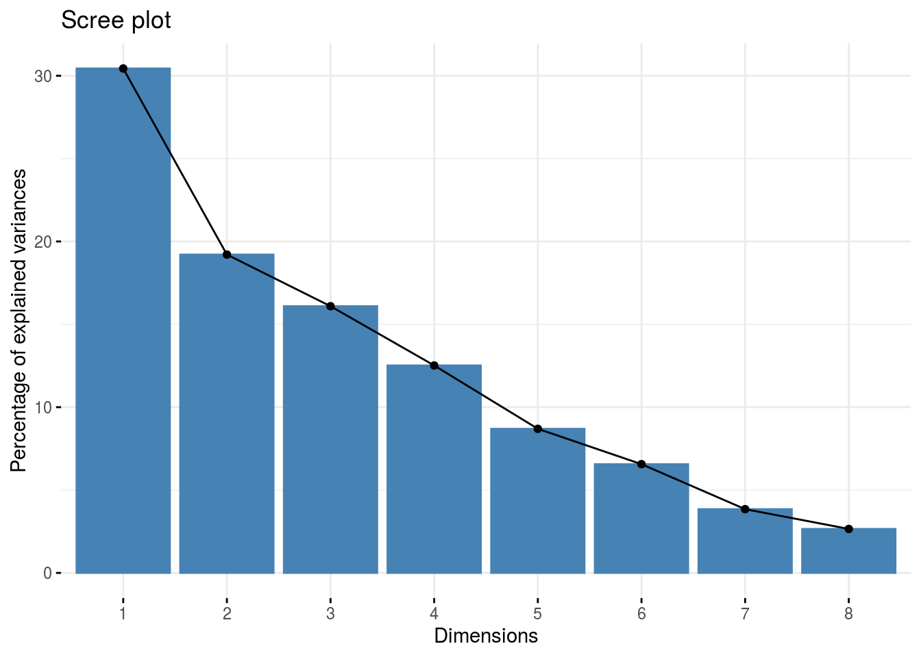
(summ.pca_sus <- summ.pca(res.pca_sus))
##              eig       diff   variance cumvariance
## Comp.1 2.4350458 0.89841649 0.30438073   0.3043807
## Comp.2 1.5366293 0.24938214 0.19207867   0.4964594
## Comp.3 1.2872472 0.28593936 0.16090590   0.6573653
## Comp.4 1.0013078 0.30586724 0.12516348   0.7825288
## Comp.5 0.6954406 0.17069972 0.08693007   0.8694588
## Comp.6 0.5247409 0.21721115 0.06559261   0.9350515
## Comp.7 0.3075297 0.09547102 0.03844121   0.9734927
## Comp.8 0.2120587         NA 0.02650734   1.0000000
fviz_pca_var(res.pca_sus,
             col.var = "contrib",
             gradient.cols = c("#00AFBB", "#E7B800", "#FC4E07"),
             repel = TRUE)
# VIF & TOL
model_sus<-lm(synthetic_opioid_crude_death_rate ~ hep_c_mortality_rate + heroin_crude_death_rate + cocaine_crude_death_rate +
                meth_crude_death_rate + heroin + tx_su + tx_mental + mental,
              data = dat.full, na.action=na.exclude)

summary(model_sus)
##
## Call:
## lm(formula = synthetic_opioid_crude_death_rate ~ hep_c_mortality_rate +
##     heroin_crude_death_rate + cocaine_crude_death_rate + meth_crude_death_rate +
##     heroin + tx_su + tx_mental + mental, data = dat.full, na.action = na.exclude)
##
## Residuals:
##     Min      1Q  Median      3Q     Max
## -56.723  -0.906  -0.190   0.647  72.751
##
## Coefficients:
##                           Estimate Std. Error t value Pr(>|t|)
## (Intercept)               -2.05668    0.32730  -6.284 3.41e-10 ***
## hep_c_mortality_rate      -0.16673    0.02092  -7.972 1.70e-15 ***
## heroin_crude_death_rate    0.34200    0.01381  24.766  < 2e-16 ***
## cocaine_crude_death_rate   1.41660    0.01888  75.024  < 2e-16 ***
## meth_crude_death_rate      0.55293    0.01864  29.665  < 2e-16 ***
## heroin                   392.41894   33.40344  11.748  < 2e-16 ***
## tx_su                    -52.05223    3.74956 -13.882  < 2e-16 ***
## tx_mental                 38.17432    2.31375  16.499  < 2e-16 ***
## mental                   -42.27898    7.43566  -5.686 1.33e-08 ***
## ---
## Signif. codes:  0 '***' 0.001 '**' 0.01 '*' 0.05 '.' 0.1 ' ' 1
##
## Residual standard error: 3.255 on 12419 degrees of freedom
##   (12428 observations deleted due to missingness)
## Multiple R-squared:  0.6471,	Adjusted R-squared:  0.6469
## F-statistic:  2847 on 8 and 12419 DF,  p-value: < 2.2e-16
##                  Variables Tolerance      VIF
## 1     hep_c_mortality_rate 0.9409307 1.062778
## 2  heroin_crude_death_rate 0.4906204 2.038236
## 3 cocaine_crude_death_rate 0.5305895 1.884696
## 4    meth_crude_death_rate 0.7786121 1.284337
## 5                   heroin 0.6449196 1.550581
## 6                    tx_su 0.8247889 1.212431
## 7                tx_mental 0.3690331 2.709784
## 8                   mental 0.4157689 2.405182