Chapter 2 Data

2.1 LIBRARIES

library(tidyverse)
library(ggmap)
library(maptools)
library(rgeos)
library(readxl)
library(sf)
library(rgdal)
library(leaflet)

2.2 ADMINISTRATIVE AND SPATIAL DATA

data <- read.csv("./_data/Cleaned_Final_Dataset_2018_7-2-20.csv", stringsAsFactors = F)

usa.sf <- st_read("./_data/GIS/tl_2017_us_county/tl_2017_us_county.shp",  stringsAsFactors = F) %>%
  #filter(STATEFP=="01") %>%
  filter(STATEFP!="02", STATEFP!="15", STATEFP!="60", STATEFP!="66", STATEFP!="69", STATEFP!="72", STATEFP!="78") %>%
  mutate(county_code = as.numeric(GEOID),
         STATEFP = as.numeric(STATEFP)) %>%
  left_join(read_excel("./_data/fp_codes.xlsx") %>%
              dplyr::rename(STATEFP = `Numeric code`), by = "STATEFP") 

## Reading layer `tl_2017_us_county' from data source `/research-home/gcarrasco/EMMERG_MAP2/_data/GIS/tl_2017_us_county/tl_2017_us_county.shp' using driver `ESRI Shapefile'
## Simple feature collection with 3233 features and 17 fields
## geometry type:  MULTIPOLYGON
## dimension:      XY
## bbox:           xmin: -179.2311 ymin: -14.60181 xmax: 179.8597 ymax: 71.43979
## CRS:            4269

usa.sf %>% 
  group_by(loc) %>%
  summarise(c = mean(county_code)) %>%
  ggplot() + 
  geom_sf(aes(fill = loc), size = 0.5, col = "black") +
  theme_bw()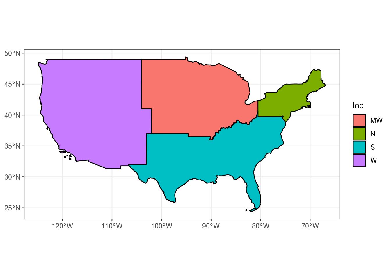

dat.sf <- usa.sf %>%
  inner_join(data, by="county_code")

2.3 Synthetic Opioid Deaths

library(colorspace)
library(ggsci)
library(ggthemes)
library(cowplot)

sd_m <- dat.sf %>% 
  ggplot() + 
  geom_sf(aes(fill=synthetic_opioid_deaths), size = 0.3, col = NA) +
  #scale_fill_continuous_sequential("BurgYl", trans = "log10", na.value = "#CDCDC1") +
  scale_fill_continuous_sequential("BurgYl", trans = "pseudo_log", na.value = "#CDCDC1", breaks = c(1,3,10,30,100,300,3000)) +
  labs(fill = "Synthetic Opioid Deaths") +
  theme_void()  +
  theme(panel.grid.major = element_line(color = "white"),
        strip.text = element_text(size=15),
        legend.position = "bottom") +
  facet_wrap(.~year,  ncol = 2)

sd_t <- dat.sf %>% 
  st_set_geometry(NULL) %>%
  group_by(year, loc) %>%
  summarise(synthetic_opioid_deaths = sum(synthetic_opioid_deaths, na.rm = T)) %>%
  rbind(dat.sf %>% 
          st_set_geometry(NULL) %>%
          mutate(loc = "US") %>%
          group_by(year, loc) %>%
          summarise(synthetic_opioid_deaths = sum(synthetic_opioid_deaths, na.rm = T))) %>%
  ggplot(aes(x = year, y = synthetic_opioid_deaths, col = loc)) +
  geom_line() +
  labs(y = "Synthetic Opioid Deaths", color = "Area") +
  scale_color_npg() +
  theme_few() +
  theme(legend.position = "bottom")

plot_grid(sd_t, sd_m, labels = c("A)", "B)"), nrow = 1)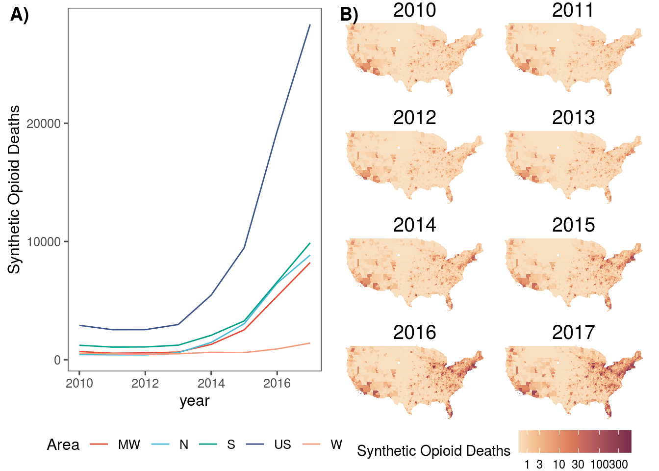

# IN TEXT
dat.sf %>% 
  st_set_geometry(NULL) %>%
  ungroup() %>%
  filter(synthetic_opioid_deaths>=10) %>%
  summarise(synthetic_opioid_deaths = sum(synthetic_opioid_deaths, nana.rm = T))

##   synthetic_opioid_deaths
## 1                   53532

dat.sf %>% 
  st_set_geometry(NULL) %>%
  ungroup() %>%
  filter(synthetic_opioid_deaths>=10) %>%
  distinct(GEOID) %>%
  count()

##     n
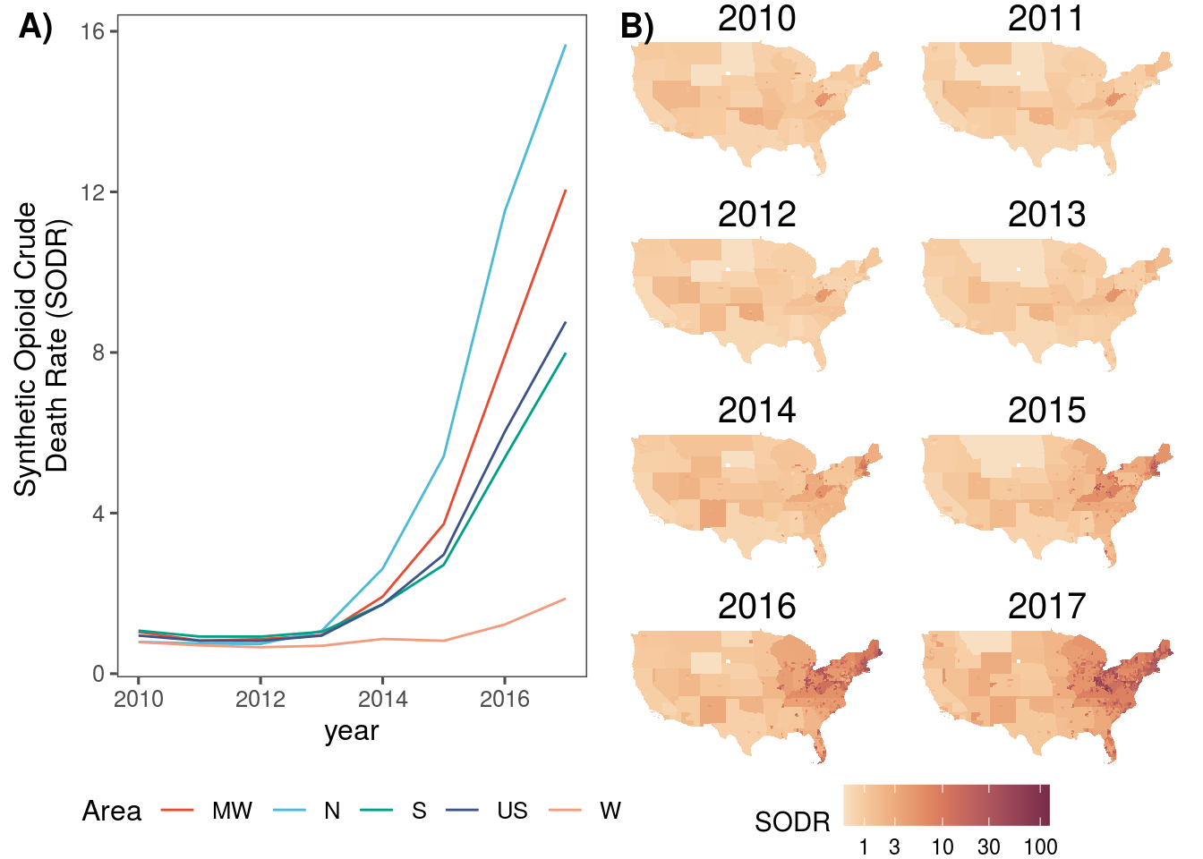
## 1 502

2.4 Synthetic Opioid Deaths Rate

library(colorspace)
library(ggsci)
library(ggthemes)
library(cowplot)

sr_m <- dat.sf %>% 
  ggplot() + 
  geom_sf(aes(fill=synthetic_opioid_crude_death_rate), size = 0.3, col = NA) +
  #scale_fill_continuous_sequential("BurgYl", trans = "log10", na.value = "#CDCDC1") +
  scale_fill_continuous_sequential("BurgYl", trans = "pseudo_log", na.value = "#CDCDC1", breaks = c(1,3,10,30,100,300,3000)) +
  labs(fill = "SODR") +
  theme_void()  +
  theme(panel.grid.major = element_line(color = "white"),
        strip.text = element_text(size=15),
        legend.position = "bottom") +
  facet_wrap(.~year,  ncol = 2)

sr_t <- dat.sf %>% 
  st_set_geometry(NULL) %>%
  group_by(year, loc) %>%
  summarise(synthetic_opioid_deaths = sum(synthetic_opioid_deaths, na.rm = T),
            population = sum(population, na.rm=T)) %>%
  rbind(dat.sf %>% 
          st_set_geometry(NULL) %>%
          mutate(loc = "US") %>%
          group_by(year, loc) %>%
          summarise(synthetic_opioid_deaths = sum(synthetic_opioid_deaths, na.rm = T),
                    population = sum(population, na.rm=T))) %>%
  mutate(synthetic_opioid_crude_death_rate = 100000*synthetic_opioid_deaths/population) %>%
  ggplot(aes(x = year, y = synthetic_opioid_crude_death_rate, col = loc)) +
  geom_line() +
  labs(y = "Synthetic Opioid Crude \nDeath Rate (SODR)", color = "Area") +
  scale_color_npg() +
  theme_few() +
  theme(legend.position = "bottom")

plot_grid(sr_t, sr_m, labels = c("A)", "B)"), nrow = 1)