3.2 Generalization and external validity evidence
3.2.1 Generalizing about a population based on a sample
When you go to an ice cream shop, you might ask for a sample of different ice cream flavors before you decide which one to get. Of course, part of the fun is getting to eat the sample! But when you ask for a sample of an ice cream, you probably want to learn more than just whether the particular bite that you tried good. You are probably interested in learning about the ice cream flavor in general. Similarly, when a chef is making a pot of soup, they might try a sample of the soup as it cooks. The point is to learn about the whole pot, by trying a sample.
These are both examples of generalizing, that is, making an inference about a larger population (an entire flavor of ice cream, an entire pot of soup), based on a sample.
Similarly, scientists and statisticians are often interested in making an inference about a larger population based on a sample. For example, in the Monday Breakups activity, our research question was about all breakups on Facebook, but our analysis was based on a random sample of 50 breakups. This is a common theme in statistical analysis. We often do not have access to the entire population that we are interested in. Instead we do the analysis on a sample and then we make an argument about why the result can be generalized beyond the sample.
Vocab
- We use the term population to refer to the group that we are interested in learning about, for example, an entire flavor of ice cream, or a whole pot of soup, or all breakups reported on Facebook.
- We use the term sample to refer to the data that we actually study. For example, the bite of ice cream or soup that we actually try, or the the sample of 50 breakups from Facebook that we actually analyzed.
3.2.2 Evaluating generalizabiltiy
Of course, it’s not always appropriate to make a generalization about a population based on a sample. Imagine trying a sample of soup from a the top of a pot that hadn’t been stirred. That sample may not be a good representation of the pot of soup, and so it would not be appropriate to make an inference about the pot based on the sample.
The same is true in statistics. Evaluating the generalizability of a result is a process of examining evidence and making a judgment. That’s something only humans can do! Statistics can’t do this for us. However, a statistical perspective can give us a disciplined way to think about generalizability. The statistical perspective on generalizability is called external validity.
To evaluate the external validity evidence in a study, statisticians examine two criteria:
Representativeness: Is the sample representative of a broader population?
Uncertainty: How much uncertainty is there, and have the researchers accounted for the uncertainty in their analysis?
To explore these ideas, we’ll use the Crazy in Love activity. In that activity, the population of interest is every word in the lyrics to Crazy in Love. Each person in class chose a sample of 5 words from the population, using two different techniques. First, you chose a purposeful sample of 5 words that, in your judgment, were representative of the lyrics in the population. Then you chose a random sample of 5 words. We then found the mean length of the words in each sample, and looked at the distribution of the mean length of the words in each sample:

Figure 3.1: The distributions of sample means for samples of 5 words
3.2.3 Sampling distributions
Take a moment to understand the distributions in Figure 3.1. Each dot represents a different sample—in particular, each dot represents the mean length of the words in the given sample. The distributions are distributions of sample statistics. We call distributions like this sampling distributions.16
Statisticians define representativeness and uncertainty based on the how sampling distributions are related to the population.
3.2.4 Comparing the sample means to the “true” population mean
For the Crazy in Love activity, we have access the whole population (all the lyrics) and therefore we could find the “true” mean of all the words in the population. The “true” mean is 3.58 letters. This is shown with a purple line in the figure below.
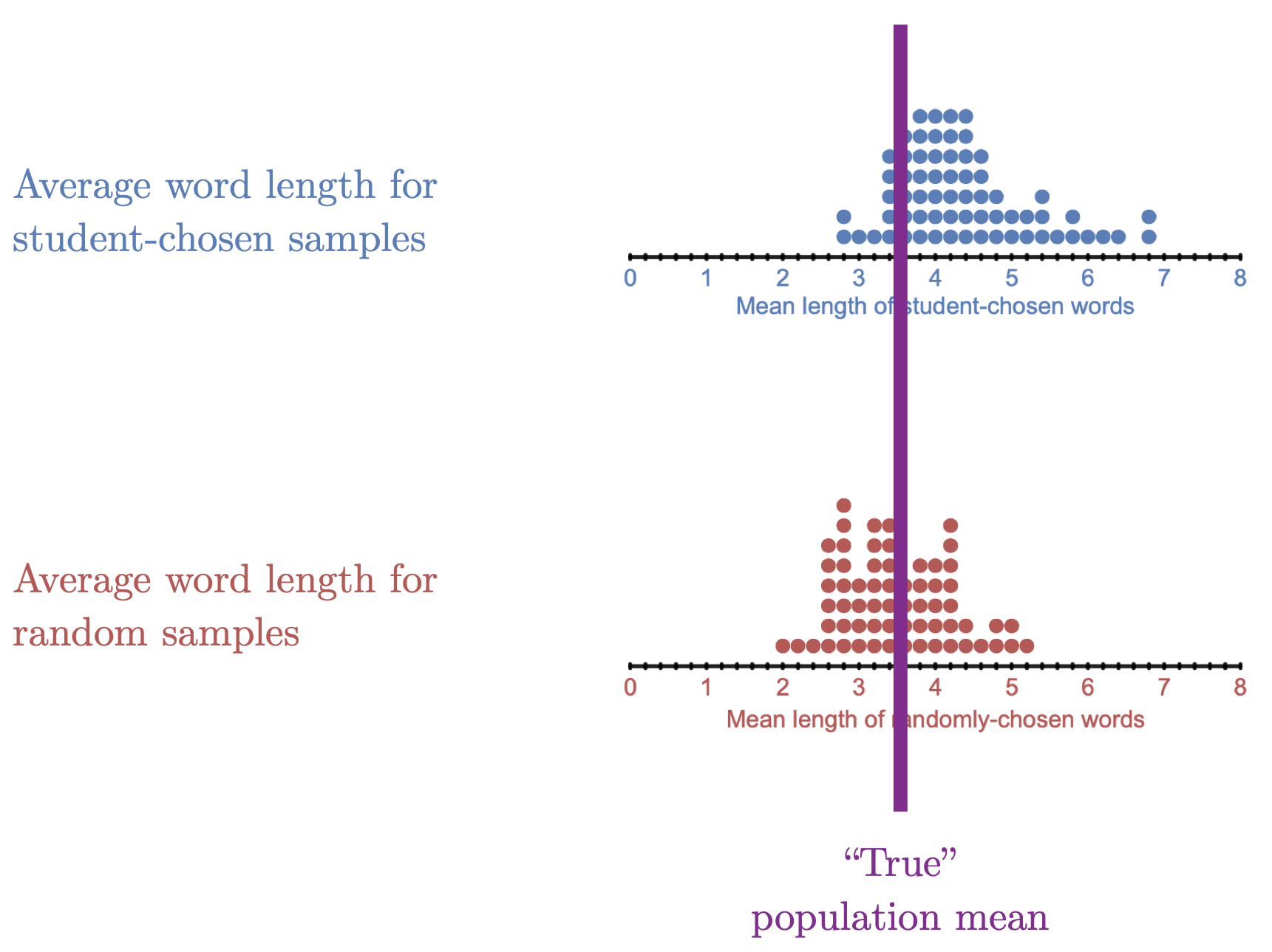
Figure 3.2: This figure is a metaphor for statistical bias.
We will use the sampling distributions in Figure 3.2 to introduce representativeness and uncertainty.
(Before we go any further, let’s point out two curious aspects of this activity. First, we had access to the population of interest. In real life, if a scientist had access to the entire population, they wouldn’t take a sample, they would just do their analysis on the population. Second, in this activity, we took a lot of different samples. In real life, scientists usually only get one sample. We’ll use this activity to learn about the key ideas behind generalizabilty, but keep in mind that this is not meant to demonstrate how analyses typically work.)
3.2.5 Representativeness and bias
Notice in Figure 3.2 that different samples sometimes had different means. Some sample means were close to the population mean, and other sample means were far from the population. Neither sampling method was perfectly accurate for every sample.
However, if we want to learn about different sampling methods, the important thing is to look at the associated sampling distributions, not at a single sample. Notice that the sampling distribution for the random samples (the red distribution) is centered at the population mean, while the sampling distribution for the purposeful samples (the blue distribution), is shifted to the right. This means that the purposeful samples systematically overemphasized longer words and under-emphasized shorter words.
3.2.5.1 Bias
Statisticians use the term bias to describe a sampling method that systematically over- or under-emphasizes a particular trait in the population.
When you take a sample of soup from the top of a pot that has not been stirred, you are using a biased sampling method, because you are systematically overemphasizing the oily bits of of the soup that have accumulated at the top. In the Crazy in Love activity, purposeful sampling was a biased sampling method because it systematically overemphasized long words.
When you take a sample from a put that has been stirred, you are using an unbiased sampling method. Stirring the soup makes it so that there is no systematic over- or under-emphasis of any aspect of the soup in your sample. Similarly, random sampling is an unbiased sampling method. Random sampling is like stirring the soup. It makes it so there is no systematic over or under-emphases in the sample. In the crazy in love activity, the random samples, on average, are accurate. And even though the random samples did not always perfectly match the mean word length in the population, they did not systematically over- or under-emphasize word lengths.
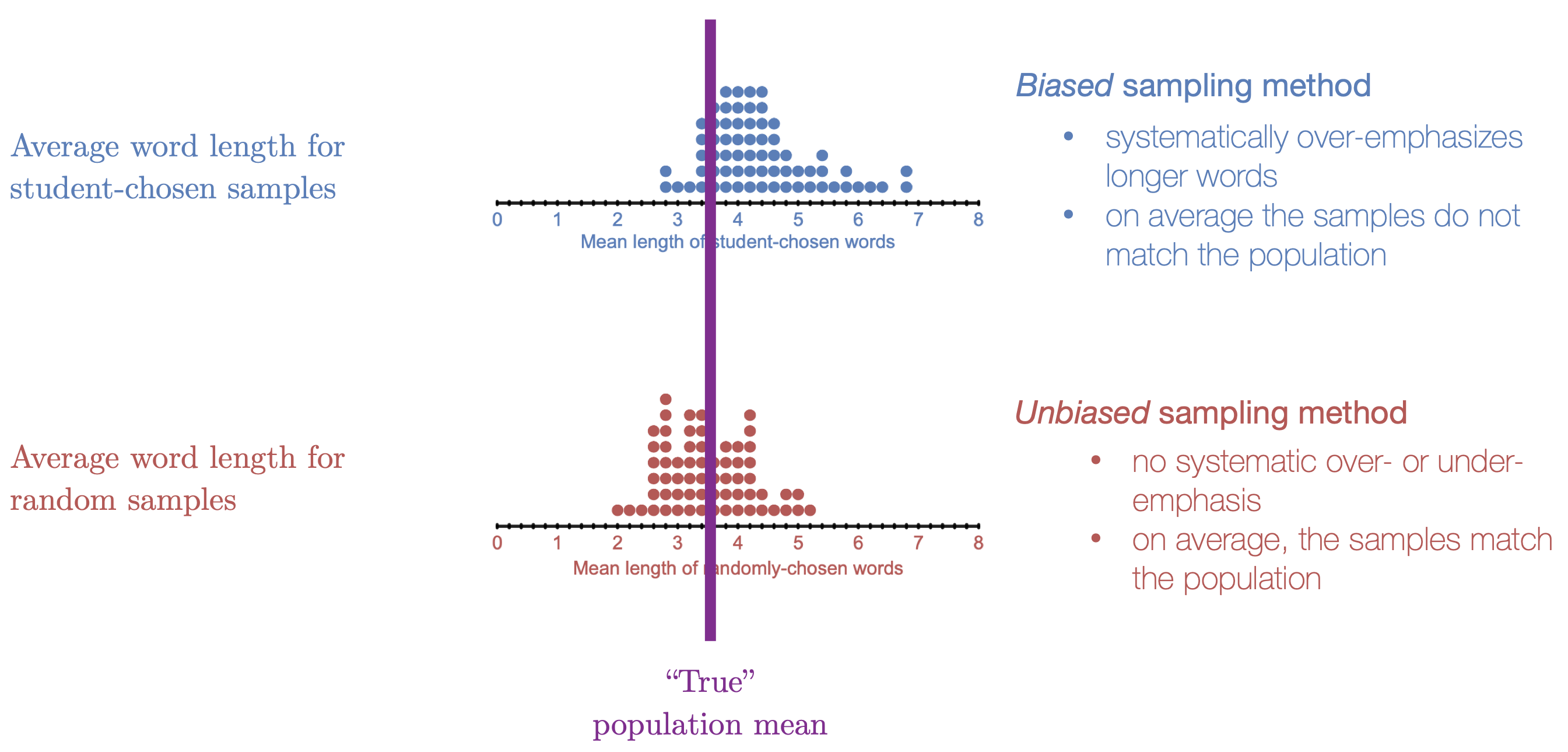
Figure 3.3: In the Crazy in Love activitiy, purposeful samping was a biased method becuase it systemaitcally over-emphasized longer words. Random samping is an unbiased sampling method.
Here are the key points about statistical bias:
- Bias is a property of the sampling method
- Bias does not necessarily mean “prejudiced” or purposefully discriminatory
- Biased does not necessarily mean the sample is wrong. It means that method is systemically inaccurate
- Unbiased does not mean the sample is “perfectly accurate.” It means, the method is not systematically inaccurate.
To summarize, when one uses a biased sampling method, a typical sample does not match the population. When one uses an unbiased sampling method, a typical sample matches the population.
Aside from purposeful sampling, there are lots of ways that bias can creep into a sampling method. Please read the link below to learn about some common sources of bias.
https://www.scribbr.com/methodology/sampling-methods/#non-probability-sampling
3.2.5.2 Representative samples and random sampling.
Statisticians define a representative sample as one that comes from an unbiased sampling method. A representative sample is not necessarily perfectly accurate. It just means that the sampling method is not systematically inaccurate and therefore samples are accurate on average. Random sampling is an unbiased sampling method that produces representative samples.
In this course, we will often discuss and utilize simple random sampling. To draw a simple random sample we need a list of EVERY member of the population. This list is called the sampling frame. Then we employ randomness to draw out sampling units, with the caveat that each unit in the sampling frame has an equal chance of being drawn.
Statisticians love random sampling because it is an unbiased sampling method that produces representative samples. However, it is often difficult to get a truly random sample. First of all, it can be difficult to obtain a sampling frame that has every member of the population. And even we have an accurate sampling frame, it is often impossible to get a truly random sample without having at least a little bit of convenience bias or volunteer bias. For example, imagine we want to learn the average amount of time that adults in the US spend watching TV. It would be very difficult to get an accurate sampling frame—try obtaining a list of everyone who lives in the United States! And then, some members of our sample may not have a phone or address. So we might skip those people and thus we have some convenience bias. And finally, some of the people we contact may refuse to answer, so we would have some volunteer bias.
We can’t just throw up our hands and reject any sample that is not truly random. Remember, determining the representativeness of a sample is a process of evaluating the evidence and making a judgment. If we don’t have a truly random sample, it’s up to the researcher to make an argument about why the sample is still representative of the population, and it’s up to the readers to evaluate that argument.
Vocab
- Statistical bias is a systematic tendency to over- or under-emphasize an attribute of the population in the sample
- A representative sample is a sample that comes from an unbiased sampling method
Key points: Represenativeness and bias
Random sampling is an unbiased sampling method that produces representative samples.
If we don’t have a random sample, we have to use human judgment to determine if the sample is representative of the population.
3.2.6 Uncertainty and sampling variation
If we have a representative sample, our samples are accurate on average. But still, not every sample is the same. Different samples give us different results. This sample-to-sample variation is called sampling variation.
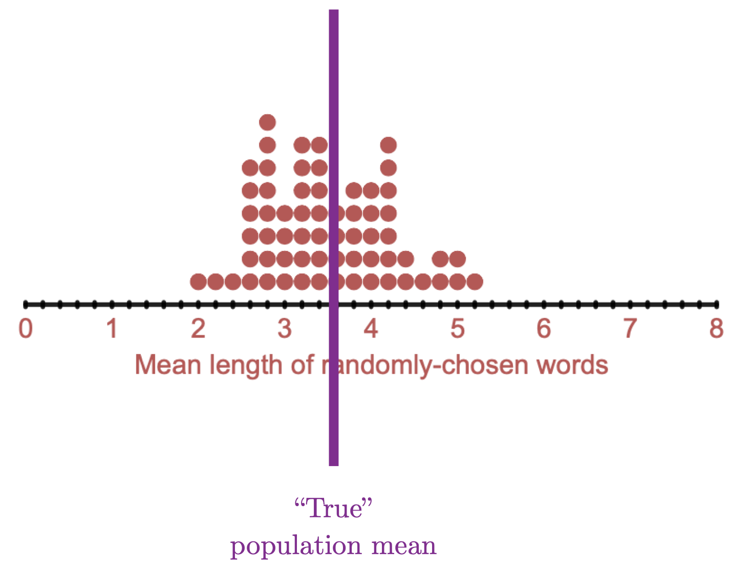
Figure 3.4: Even though we have an unbiased sampling method, there is still sampling variabilty.
Because of sampling variation, there is always uncertainty when we generalize from a sample to a population. We may have a sample that perfectly matches the population, or we may have a sample that “misses” the true value in the population. This uncertainty due to sampling variation is unavoidable. We can’t eliminate it. Instead we have to account for it in our analysis.
To account for uncertainty due to sampling variability, we need to know how much variability there is from sample to sample. This is just what Monte Carlos simulation can tell us! In fact, the reason we do a hypothesis test is to account for the uncertainty due to sampling variation!
When we do a hypothesis test, we simulate multiple samples that are compatible with the null hypothesis. The SD of the distribution of simulated results is a measure of sampling variation if the null hypothesis were true. When we find a p-value, we are finding the probability of obtaining our observed result just by sampling variation if the null hypothesis were true. Thus a p-value is a measure of uncertainty. The lower the p-value the less uncertainty we have in our result due to sampling variation
Vocab
- Sampling variation is the unavoidable variability from sample to sample
Key points: Uncertainty and sampling variation
Sampling variation leads to uncertainty when we generalize from a sample to a population
We have to account for the uncertainty due to sampling variation, for example, by doing a hypothesis test.
3.2.7 Putting it together
Generalizability is the extent to which it is reasonable to make an inference about a population based on a sample. The statistical perspective on generalizability is called external validity.
To evaluate the external validity evidence in a study, we examine two criteria:
Representativeness: Is the sample representative of a broader population? Here, consider bias in the sampling method. What are the sources of bias, and are they likely to have a systematic effect on the attribute of interest?
Uncertainty: How much uncertainty due to sampling variation is there, and have the researchers accounted for the uncertainty in their analysis? One way that researchers account for uncertainty due to sampling variation is by doing a hypothesis tests. The p-value is a measure of the uncertainty due to sampling variation.
Altogether, we can evaluate the external validity evidence of a study on a continuum. If the sample is not representative of a broader population, the case for generalizing is weak. If the sample is representative, consider the uncertainty due to sampling variation.
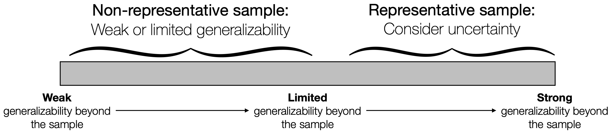
Figure 3.5: We can rate the external validity evidence on a continuum by considering representativeness and uncertainty.
3.2.8 Example 1: Monday breakups
In the Monday breakups activity, our research question was:
Are breakups on facebook more likely to be reported on Monday?
Based on the research question, the population that we are interested is all breakups on facebook.
Our sample is a random sample of 50 breakups from facebook.
The observed result in the sample was: 13/50 (26%) of breakups were reported on Monday.
The conclusion from the hypothesis test was: The observed sample data is not compatible with a null hypothesis where breakups are equally likely each day (p=0.016). This suggests that breakups are more likely to be reported on Monday.
This conclusion is based on a sample of 50 breakups. Can the results be generalized to all breakups on facebook? To answer this question, we examine the external validity evidence, including representativenss and uncertainty.
Representativeness
Is the sample representative of a broader population?
Yes. This study used a random sample of breakups from the population of interest (all breakups on facebook). Random sampling is an unbiased sampling method, which means that the sample is representative of the population.
Uncertainty due to sampling variation
Have the researchers accounted for uncertainty due to sampling variation?
Yes. The hypothesis test accounts for uncertainty due to sampling variation. Recall that, if the null hypothesis were true, we would expect 14% of breakups in our sample to be reported on Monday. But we didn’t compare the observed result (26% of breakups in the sample were reported on Monday) to the expected result if the null hypothesis were true (14% of breakups would be reported on Monday). This is because we had to account for sampling variation. Even if the null hypothesis were true, a random sample of 50 breakups may not have exactly 14% of breakups on Monday. We accounted for sampling variation two ways: by computing the range of likely results if the null hypothesis were true and comparing our observed result to this range, and by computing a p-value. Because the observed result is outside the range of likely results if the null hypothesis were true (or, because the p-value is low), we are confident in our conclusion even with the uncertainty due to sampling variation.
Conclusion
Because we have a representative sample and because we have accounted for uncertainty due to sampling variation, we have a strong case that the result can be generalized to all breakups on facebook. On the external validity evidence continuum:
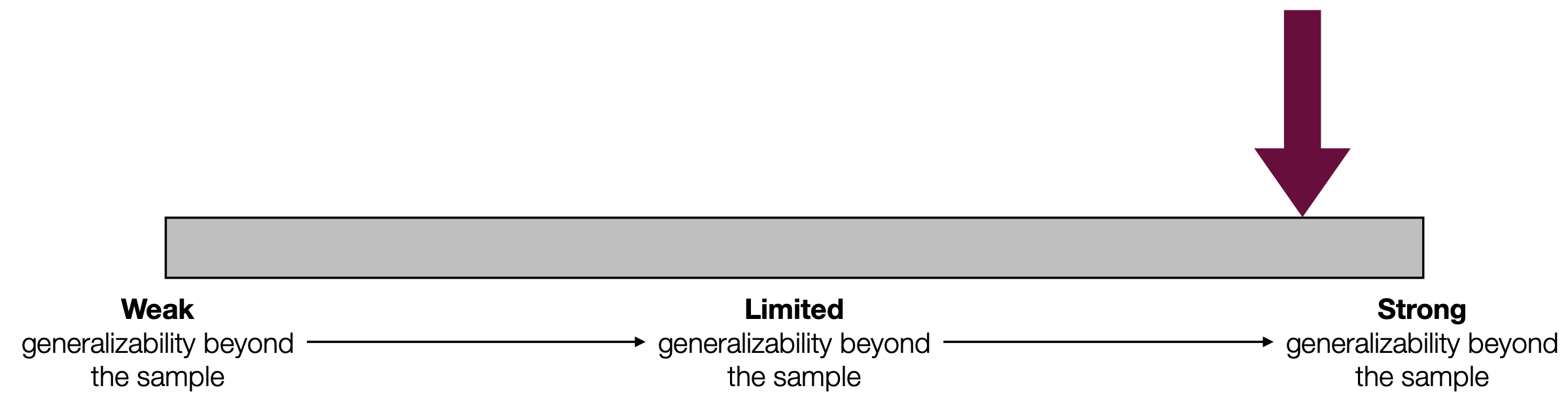
Figure 3.6: In the Monday breakups activity we had a representative sample and we accounted for uncertainty due to sampling variation by doing a hypothesis test.
3.2.9 Example 2: Racial disparities in police stops
In the Racial disparities in police stops activity, our research question was:
Does the percentage of black drivers being stopped provide evidence of possible racial disparities?
Our sample is a all 105 traffic stops made on Halloween 2017, in Minneapolis.
Based on the research question, it is difficult to determine the population of interest. We may only be interested in the police stops on Halloween 2017, in Minneapolis. Or perhaps we are interested in making a broader claim about traffic stops.
The observed result in the sample was: 39/105 (37.1%) of stopped drivers were black.
The conclusion from the hypothesis test was: The observed sample data is not compatible with a null hypothesis where there is no racial disparity in police stops (p=0.002). This suggests that there are racial disparities in the police stops on Halloween 2017 in Minneapolis.
Notice that our conclusion is limited to the sample data: The police stops in Minneapolis on Halloween 2017. Can the results be generalized beyond the sample? To answer this question, we examine the external validity evidence, including representativenss and uncertainty.
Representativeness
Is the sample representaitve of a broader population?
Maybe—but we should be skeptical. Our sample is not a random sample from a broader population, instead it is a convenience sample. This means that there is convenience bias, and thus the sample may not be representative of a broader population in terms of racial discrepancies in police stops. For example, maybe police in Minneapolis are systematically different from police in other cities with respect to racial discrepancies in police stops. Or maybe police in large cities are systematically different from police in suburban or rural areas. Or maybe the behavior of drivers on Halloween is systematically different from their behavior on other nights. Or maybe police behavior has changed since 2017, so the sample is systematically different from police behavior today. Because we don’t have a random sample, there is the potential for the sampling method to be biased in these and other ways.
The question is whether any of these potential biases is plausible, or whether or sample is reasonably representative of a broader population with respect to racial discrepancies in police stops. This is where human judgement comes in. There are reasonable arguments to be made on each side. For me, I think it is reasonable that our convenience sample may be systematically different from a broader population, so I would say that the sample is not representative of a broader population. However, a reasonable argument could be made in support of representativeness as well.
Uncertainty due to sampling variation
Have the researchers accounted for uncertainty due to sampling variation?
Yes. The hypothesis test accounts for uncertainty due to sampling variation. Recall that, if the null hypothesis were true, we would expect 18.6% of stopped drivers to be Black. We didn’t compare the observed result (37.1% of stopped drivers were Black) to the expected result if the null hypothesis were true (18.6% of stopped drivers would be Black). This is because we had to account for sampling variation. Even if the null hypothesis were true, there is some randomness in police stops, so a sample of 105 police may not match the demographics of the city exactly. We accounted for sampling variation two ways: by comparing our observed result to the range of likely results if the null hypothesis were true, and by computing a p-value. Because the observed result is outside the range of likely results if the null hypothesis were true (or, because the p-value is low), we are confident in our conclusion even with the uncertainty due to sampling variation.
Conclusion
The results of the hypothesis test suggest that there is a racial discrepancy in police stops on Halloween 2017 in Minneapolis. However, because the data come from a convenience sample and because there are plausible reasons to suspect that convenience bias may render the sample systematically different from a broader population of police stops, the case for generalizing beyond the sample is fairly weak:
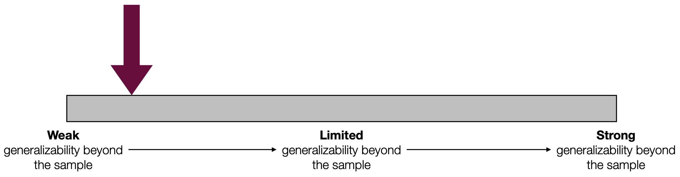
Figure 3.7: In the Racial disparities in police stops activity, there is reason to suspect that convenience bias renders the sample non-representative of a broader population, so the case for generalization is weak.
Thus, I would argue that it is not appropriate to make a claim about policing in general based on this one study.
One way to improve the case for generalizabilty is to do this study in multiple different contexts. If the results were similar in different demographic areas on different days, then the argument for generalizability is strengthened. On the other hand, if the results seem to vary across contexts, than we would learn that context matters, and that we should be skeptical of generalizing results beyond their specific contexts. Either way, even if this study can’t support a broad claim on its own, it can serve as part of a body of evidence that helps us learn more about race and policing.
More generally, even if the results from a study that involves a non-representative sample can’t be generalized on their own, the results from these studies can be used as part of a body of evidence that collectively either makes an argument for generalizability or gives a more nuanced perspective on generalizability.