1.8 Linear regression
Remember the distinction between a mathematical world and a statistical world? In a mathematical world, we are interested in how the value of one variable is associated with another variable. In a statistical world, we are interested in how the distribution of one variable is associated with another variable.
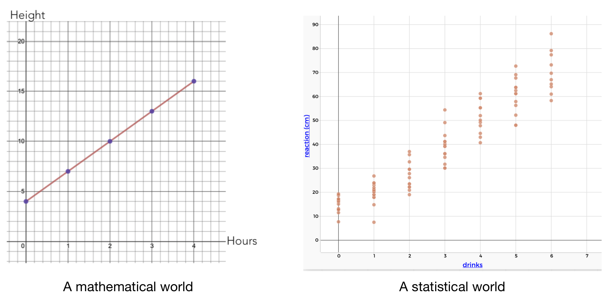
Figure 1.16: Comparing mathematical and statistical worlds
1.8.1 Summarizing a liner assocation in a mathematical world
In a mathematical world, we can summarize a linear relationship between two variables with a linear equation. For example, the graph below shows the height of a pool over time as it is being filled. There is a linear relationship between the height of the water and time.
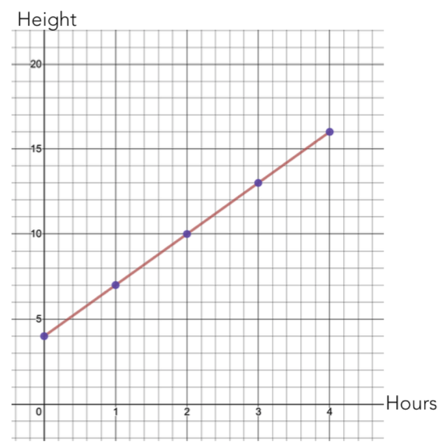
Figure 1.17: Mathematical association between height and time
Looking at the graph, we can see a few things. First of all, at \(time=0\), the height of the pool was 4ft. Then, for every 1 hours that passes, the height of the water increases by 3ft. We can summarize this using an equation:
\[height=4+3 \times hours\] In this equation:
- the \(4\) is called the intercept. It represents the hight of the pool when \(time=0\). This is sometimes called the “starting value.”
- The \(3\) is called the slope. It represents the rate at which the pool height is increasing.
1.8.2 Summarizing a liner assocation in a statistical world
In a statistical world, we are interested in how the distribution of one variable is associated with another. For example, how is the distribution of reaction times associated with alcohol consumption?
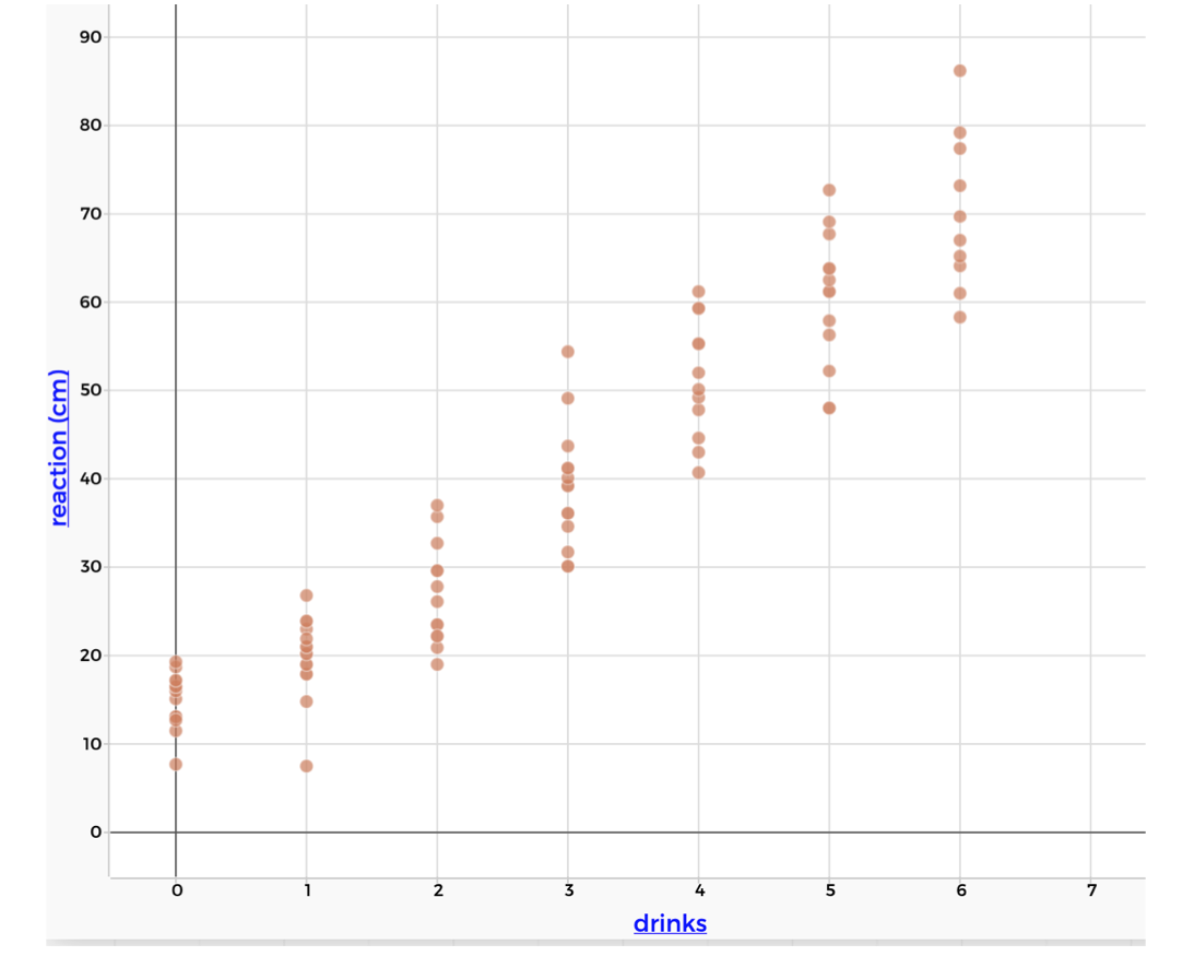
Figure 1.18: Statistical association between alcohol and reaction time
Even though we can’t connect the points with a straight line, the distributions seem to be following a liner pattern. It seems that as the number of drinks increases by 1, the reaction increases by about 10cm. This is even more apparent if we look at the typical value (the mean) of each distribution.
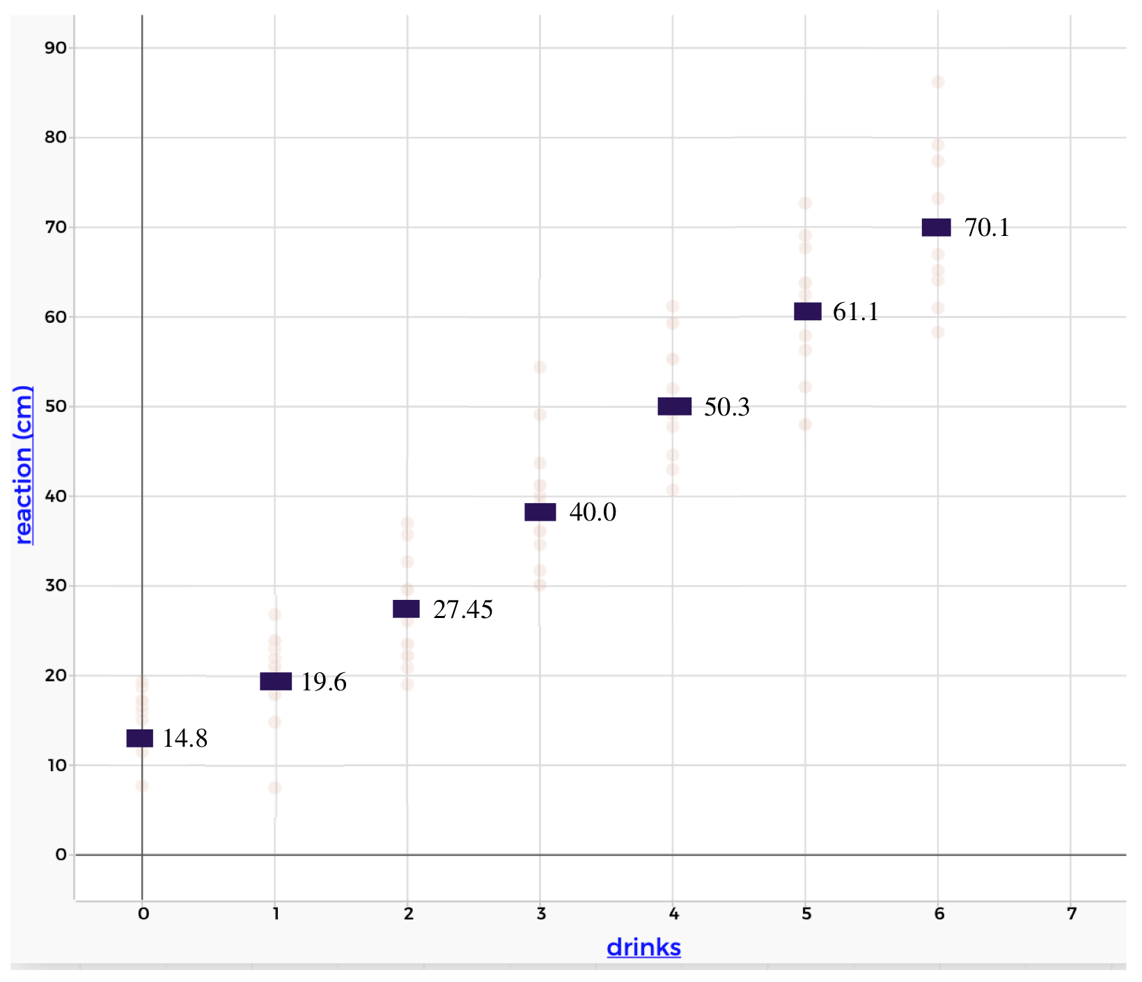
Figure 1.19: The association between alcohol and reaction time, with the means of each distribution highlighted
We can summarize this linear relationship using a linear regression. This finds the straight line that is the best summary of the statistical association. The figure below shows the regression line for the alcohol and reaction time data:
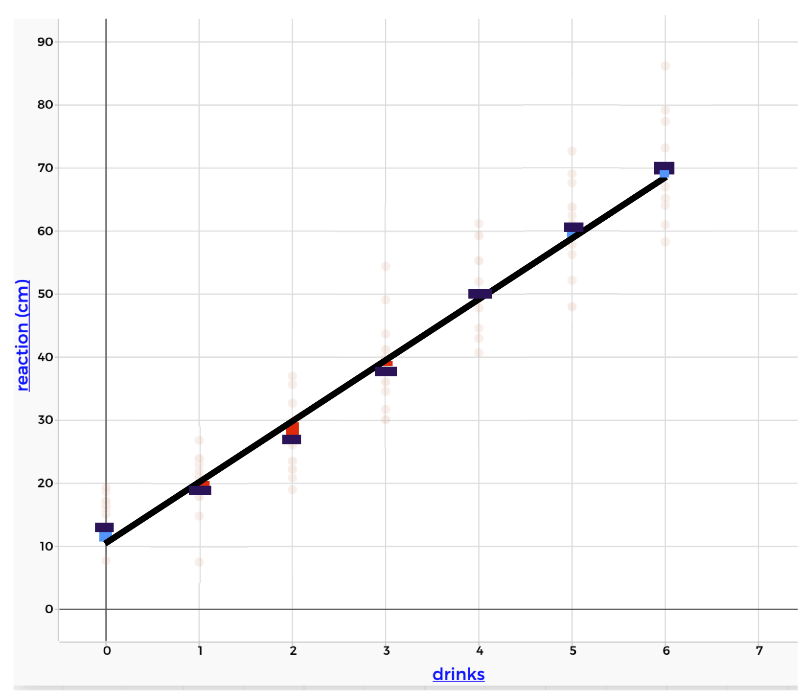
Figure 1.20: A linear regression line for alcohol and reaction time
Notice that the line doesn’t fit the mean of the distributions perfectly, but it’s pretty close. The deviations from the line to the means are marked in red and blue. The linear regression line balances these deviations (if you add up the red deviations, it would be equal to the blue deviations). This means that the line is not biased towards overestimating the means or underestimating the means. It is often called a “line of best fit.”
The equation for this line is:
\[reaction = 11.3 + 9.7 \times drinks\] Just like in the mathematical world, there is an intercept and a slope. These have a similar interpretation in the statistical world. However, we have to remember that we are summarizing the behavior of distributions. We communicate that using words like “approximately” and “on average” and “we expect.”
- The intercept is 11.3. This means that, on average, we expect the reaction to be approximately 11.3cm when the participant has had 0 drinks.
- The slope is 9.7. This means that, on average, when the number of drinks increases by 1, we expect the reaction to increase by approximately 9.7cm.
Linear regression
- The linear regression is a mathematical model of a liner statistical association
- The line is called a “line of best fit”
- The intercept tells us the typical value of the y-variable, when the x-variable is 0
- The slope tells us how much we expect the y-variable to increase, on average, for every 1-unit increase in the x-variable.
| Resources |
|---|
| ⏯ How to find a linear regression in TinkerPlots |