Chapter 7 One Sample t-Test

Now that we have gone over the simple linear regression and how the simple linear regression is written and interpreted identically to the GLM (in addition to its standardized counterpart, the correlation), we can begin covering the other statistical analyses in the order they are typically taught.

Let’s now go over the one-sample t-test, which compares a sample mean to a population mean (or an a priori value).

For example, let’s say we were interested in determining if the salary of professors was significantly different than the national U.S. median income of $50,221 in 2009.

For this example, we will again be using the datasetSalaries dataset.

7.1 Null and research hypotheses

7.1.1 Traditional Approach

\[H_0: \mu = \$50,221\] \[H_1: \mu \ne \$50,221\]

where \(\mu\) represents the population mean

The null hypothesis states that there is no difference between the sample and population mean, or equivalently the sample and population mean are equal. The research hypothesis states that there is a difference between the sample and population mean, or equivalently the sample and population mean are not equal.

7.1.2 GLM Approach

\[Model: Salary = \beta_0 + \varepsilon\] \[H_0: \beta_0 = \$50,221\] \[H_1: \beta_0 \ne \$50,221\]

where \(\beta_{0}\) represents the intercept, \(\varepsilon\) represents the population error, \(H_0\) represents the null hypothesis, and \(H_1\) represents the research hypothesis.

In this particular case, we will not be using the nil hypothesis as we have an a priori comparison of $50,221.

In the model, when there is no other predictor, the intercept will be the mean. This is because without any other information, the single best number to describe the data is the mean. Thus, the null hypothesis states the intercept (or the mean of 9-month academic salary of professors) is equal to $50,221. The research hypothesis states that the intercept (or the mean 9-month academic salary of professors) is not equal to $50,221.

7.2 Statistical analysis

7.2.1 Traditional Approach

To perform the traditional one-sample t-test, we can use the t.test() function. The first input is the DV of salary, which is again prefixed by the name of the dataset and the dollar sign. The second input is the a priori value (or population value, \(\mu\)) that we are interested in testing (i.e., $50,221).

t.test(x = datasetSalaries$salary, mu = 50221)

## 
##  One Sample t-test
## 
## data:  datasetSalaries$salary
## t = 41.762, df = 396, p-value < 2.2e-16
## alternative hypothesis: true mean is not equal to 50221
## 95 percent confidence interval:
##  110717.9 116695.1
## sample estimates:
## mean of x 
##  113706.5

From this output, we can see that the t-statistic (t) is 41.762, degrees of freedom (df) is 396, and the p-value is 2.2e-16, with professor’s mean salary at $113,706.50. Therefore, professors earn a significantly higher salary compared with the national U.S. median income of $50,221 in 2009.

The t-statistic and its respective p-value can be interpreted as we previously saw in the simple linear regression chapter. We will spend more time explaining these values in the next section.

7.2.2 GLM Approach

Since we have an a priori hypothesis (i.e., median income of $50,221), we will need to first manipulate the DV by point deviating from this a priori value. To do this, we will need to subtract $50,221 from each salary score. Luckily, we can do that directly within the lm() fucntion. We have to point-deviate because the lm() function always tests regression estimates including the intercept against 0 (\(H_0 = 0\)). By point deviating from $50,221, we are now asking if the mean of the new point deviated scores is different than 0, where 0 now equals $50,221. To test the intercept, we simply place a 1 as the predictor.

model <- lm(salary - 50221 ~ 1, datasetSalaries)

We will again only look at the coefficients table using the summary() function for this test and subsequent t-tests. Although, the ANOVA source table is not typically associated with this test, we could always examine it if desired using the Anova() function.

summary(model)

## 
## Call:
## lm(formula = salary - 50221 ~ 1, data = datasetSalaries)
## 
## Residuals:
##    Min     1Q Median     3Q    Max 
## -55906 -22706  -6406  20479 117839 
## 
## Coefficients:
##             Estimate Std. Error t value Pr(>|t|)    
## (Intercept)    63486       1520   41.76   <2e-16 ***
## ---
## Signif. codes:  0 '***' 0.001 '**' 0.01 '*' 0.05 '.' 0.1 ' ' 1
## 
## Residual standard error: 30290 on 396 degrees of freedom

Notice that in both approaches that the values are identical with respect to the place of rounding. The t-statistic is 41.76 with 396 degrees of freedom (df), and the p-value is <2e-16. However, the estimate of the GLM approach is now the sample mean of the point deviated scores. Thus, we if add back $50,221, we will obtain the same sample mean of $113,707⁸.

Let’s go over the t-statistic and p-value to reinforce these concepts.

Remember that the t-statistic represents the systematic difference compared to the unsystematic difference. In this case, the systematic difference is the difference between professor’s mean salary and U.S. median income (i.e., $113,707 - $50,221) and the unsystematic difference is standard error of the mean of the sample (in other words, random variability in the sample).

Also, the p-value represents the probability of finding a particular t-statistic or t-statistic more extreme assuming that the null hypothesis is true. In this case, the probability of finding a t-statistic of 41.76 or more extreme is <2.2e-16, which is extremely small and not likely to occur by chance.

7.3 Statistical decision

Given that the p-value of 2.2e-16 is smaller the alpha level (\(\alpha\)) of 0.05, we will reject the null hypothesis.

7.4 APA statement

A one sample t-test was performed to test if the salary of professors was different than the national U.S. median of $50,221. Professor salaries (M = $113,706, SD = $30,289) were significantly higher than the national U.S. median income, t(396) = 41.76, p < .001.

7.5 Visualization

# calculate descriptive statistics along with the 95% CI
dataset_summary <- datasetSalaries %>%
  dplyr::summarize(
    mean = mean(salary),
    sd = sd(salary),
    n = n(),
    sem = sd / sqrt(n),
    tcrit = abs(qt(0.05 / 2, df = n - 1)),
    ME = tcrit * sem,
    LL95CI = mean - ME,
    UL95CI = mean + ME
  )

# plot
ggplot(datasetSalaries, mapping = aes("", salary)) +
  geom_jitter(alpha = 0.1, width = 0.1) +
  geom_hline(
    yintercept = 50221,
    alpha = .5,
    linetype = "dashed"
  ) +
  geom_errorbar(
    data = dataset_summary,
    aes(
      y = mean,
      ymin = LL95CI,
      ymax = UL95CI
    ),
    width = 0.01,
    color = "#3182bd"
  ) +
  geom_point(
    data = dataset_summary, aes("", mean),
    size = 2,
    color = "#3182bd"
  ) +
  labs(
    x = "0",
    y = "9-Month Salary (USD)"
  ) +
  theme_classic() +
  scale_y_continuous(labels = scales::dollar)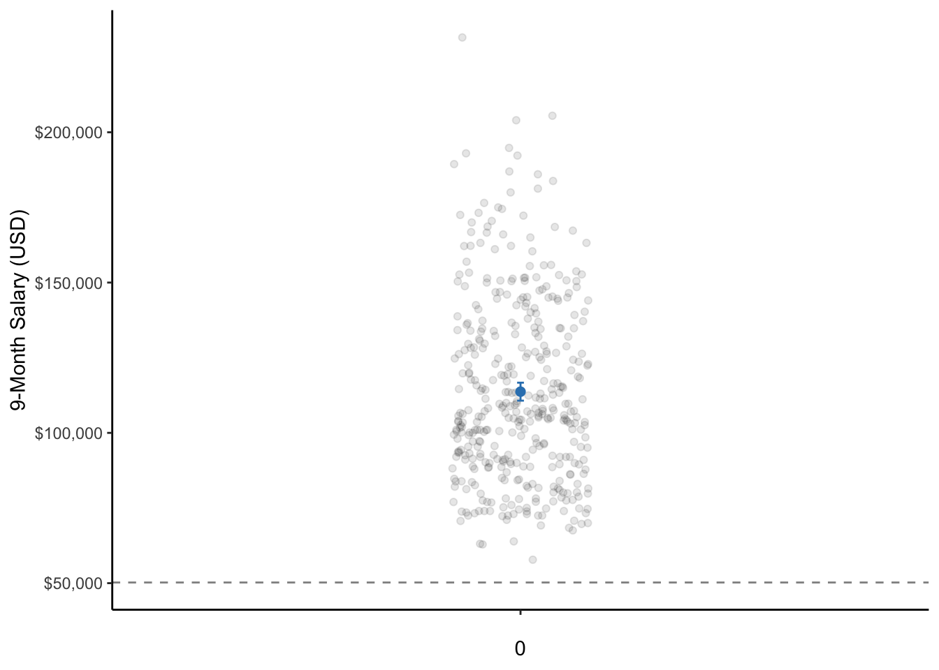

Figure 7.1: A dot plot of the salary of professors where the dot is the mean salary of professors and the whiskers are the 95% CI. Note: The data points are actually only on a single line on the x-axis. They are only jittered (dispersed) for easier visualization of all data points.

---

8. \(M = \$63,486+\$50,221=\$113,707\)↩