Chapter 9 Independent Samples t-Test

The independent samples t-test compares the means of two different (or independent) samples.

For example, let’s say that we were interested in determining if the salary of professors was different depending on whether they were part of an applied or theoretical discipline.

For this example, we will use the datasetSalaries data set.

9.1 Null and research hypotheses

9.1.1 Traditional approach

$H_0: \mu_{Applied} - \mu_{Theoretical} = 0$ or equivalently $\mu_{Applied} = \mu_{Theoretical}$
$H_1: \mu_{Applied} - \mu_{Theoretical} \ne 0$ or equivalently $\mu_{Applied} \ne \mu_{Theoretical}$

The null hypothesis states there is no difference in the salary of professors who are in an applied discipline compared to a theoretical discipline. The research hypothesis states there is a difference in the salary of professors who are in an applied discipline compared to a theoretical discipline.

9.1.2 GLM approach

\[Model: Salary = \beta_0 + \beta_1*Discipline + \varepsilon\] \[H_0: \beta_1 = 0\] \[H_1: \beta_1 \ne 0\]

In addition to the intercept ($\beta_0$), we now have a predictor discipline along with its associated slope ($\beta_1$). In this model, the slope represents the change in salary over the change in discipline, and the intercept ($\beta_{0}$) represents the value when discipline is 0.

The null hypothesis states that the slope associated with discipline is equal to zero. In other words, there is no difference in the salary of professors who are in different disciplines. The alternative hypothesis states that the slope associated with discipline is not equal to zero. In other words, there is a difference in the salary of professors that are in different disciplines.

The interpretation of the slope and intercept depends on how discipline is coded. Thus, it is always a good idea to check how this categorical IV is coded, which can be done using the contrasts() function.

contrasts(datasetSalaries$discipline)

##             Theoretical
## Applied               0
## Theoretical           1

We can see that Applied is coded as 0 and Theoretical is coded as 1. Given, that the difference of coding scheme of discipline is 1, the slope represents the mean difference in salary for professors that are in theoretical disciplines compared to applied disciplines.⁹ Additionally, the intercept ($\beta_{0}$) represents the mean salary of professors in the applied discipline since 0 represents Applied in the discipline coding scheme.

If we wanted to change the coding scheme and code Theoretical as 0 and Applied as 1, then our interpretation of the intercept would be the mean salary of professors in the theoretical discipline since Theoretical is now 0. The slope would still have the same interpretation of the mean difference of salary for professors in different disciplines as the difference in the coding scheme is still 1. However, the sign would change.¹⁰

These two types of coding schemes are known as dummy coding, which is R’s default coding scheme for categorical variables. Specifically, dummy coding is when one level of an IV is coded as 1 and all others are coded as 0. However, there are other coding schemes such as effects (also known deviant), helmert, polynomial, and orthogonal. For a good description of different contrasts in addition to applying and interpreting them, check out UCLA Statistical Consulting Group’s description. We will also go over coding categorical variables in more detail in the next chapter.

Our preferred contrast for the independent samples t-test is to use -0.5 for one group and 0.5 for the other group. We prefer this coding scheme because the slope will still provide the mean difference;¹¹ however, since 0 lies in between the two groups, the intercept will now represent the mean of the group means. In this example case, it will be the mean of the mean salary of professors in the applied discipline and the mean salary of professors in the theoretical discipline.

We recommend assigning the group expected to have a higher value in the dependent variable as 0.5 and the other group as -0.5. In our example, we might expect that those in the applied discipline will have higher salaries and thus assign that group to 0.5, while the theoretical discipline to have lower salaries and thus assign them to -0.5. We can do this by using the concatenate c() function to group the numbers together and assign them back to the contrast. The order inside the c() function must be in alphanumerical order of the levels of the independent variable.

contrasts(datasetSalaries$discipline) <- c(0.5, -0.5)
contrasts(datasetSalaries$discipline)

##             [,1]
## Applied      0.5
## Theoretical -0.5

Note: If the difference in discipline was not equal to 1, the estimate would equal the fraction of the difference. For example, if Applied was coded as -1 and Theoretical was coded as 1, the difference of discipline is now 2 and the estimate would represent half of the salary mean difference.¹² Thus, if we multiplied the estimate by 2, we would obtain the mean salary difference. Even though the estimate changes, the t-statistic and p-value will not change as the intercept and error will adjust proportionally to the coding scheme of the categorical IV (as long as they are unique values).

9.2 Statistical analysis

9.2.1 Traditional approach

To perform the traditional independent samples t-test, we can again use the t.test() function. However, we will now enter the formula of the GLM into the first argument. For this test, we will assume the variances of each group are equal (not significantly different from each other); however, this should be tested.

t.test(datasetSalaries$salary ~ datasetSalaries$discipline, var.equal = TRUE)

## 
##  Two Sample t-test
## 
## data:  datasetSalaries$salary by datasetSalaries$discipline
## t = 3.1406, df = 395, p-value = 0.001813
## alternative hypothesis: true difference in means is not equal to 0
## 95 percent confidence interval:
##   3545.70 15414.83
## sample estimates:
##     mean in group Applied mean in group Theoretical 
##                  118028.7                  108548.4

Note: There are other ways to enter the formula into t.test() function depending on how the dataset is formatted.

From this output we can see that the t-statistic (t) is 3.1406, degrees of freedom (df) is 395, and p-value is 0.001813, with the mean salary of professors in the Applied discipline being $118,028.70 and the mean salary of professors in the Theoretical discipline being $108,548.40. Therefore, professors with Applied disciplines earn significantly higher salaries than professors with Theoretical disciplines.

9.2.2 GLM approach

model <- lm(salary ~ 1 + discipline, datasetSalaries)

summary(model)

## 
## Call:
## lm(formula = salary ~ 1 + discipline, data = datasetSalaries)
## 
## Residuals:
##    Min     1Q Median     3Q    Max 
## -50748 -24611  -4429  19138 113516 
## 
## Coefficients:
##             Estimate Std. Error t value Pr(>|t|)    
## (Intercept)   113289       1509  75.060  < 2e-16 ***
## discipline1     9480       3019   3.141  0.00181 ** 
## ---
## Signif. codes:  0 '***' 0.001 '**' 0.01 '*' 0.05 '.' 0.1 ' ' 1
## 
## Residual standard error: 29960 on 395 degrees of freedom
## Multiple R-squared:  0.02436,    Adjusted R-squared:  0.02189 
## F-statistic: 9.863 on 1 and 395 DF,  p-value: 0.001813

Notice that in both analyses, the t-statistic (t value) of -3.14 with 395 degrees of freedom (df), and p-value of .002 are identical to the output from the t.test() function.

We can also see that if we subtract the mean salary for professors in the theoretical discipline from the applied discipline from the t.test() results, we obtain the same mean difference in the estimate in the GLM results (i.e., $118,028.70 - $108,548.40 = $9,480.30).

Furthermore, we can also see that the intercept is the mean of the mean salary from both those in the applied discipline and theoretical discipline ($\frac{118028.70+108548.40}{2} = 113288.50$).

9.3 Statistical decision

Given the p-value of .002 is less than the alpha level ($\alpha$) of 0.05, we will reject the null hypothesis.

9.4 APA statement

An independent samples t-test was performed to test if salary of professors was different depending on their discipline. The salary of professors was significantly higher for professors in applied disciplines (M = $118,029, SD = $29,459) than for professors in theoretical disciplines (M = $108,548, SD = $30,538), t(395) = -3.14, p = .002.

9.5 Visualization

# calculate descriptive statistics along with the 95% CI
dataset_summary <- datasetSalaries %>%
  mutate(discipline = ifelse(discipline == "Applied", 0.5, -0.5)) %>%
  group_by(discipline) %>%
  summarize(
    mean = mean(salary),
    sd = sd(salary),
    n = n(),
    sem = sd / sqrt(n),
    tcrit = abs(qt(0.05 / 2, df = n - 1)), 
    ME = tcrit * sem,
    LL95CI = mean - ME,
    UL95CI = mean + ME
  )

mean_of_means <- mean(dataset_summary$mean)

# plot
datasetSalaries %>%
  mutate(discipline = ifelse(discipline == "Applied", 0.5, -0.5)) %>%
  ggplot(., aes(discipline, salary)) +
    geom_jitter(alpha = 0.1, width = 0.05) +
    geom_line(data = dataset_summary, aes(x = discipline, y = mean), color = "#3182bd") +
    geom_errorbar(data = dataset_summary, aes(x = discipline, y = mean, ymin = LL95CI, ymax = UL95CI), width = 0.02, color = "#3182bd") +
    geom_point(data = dataset_summary, aes(x = discipline, y = mean), size = 3, color = "#3182bd") +
    geom_point(aes(x = 0, y = mean_of_means), size = 3, color = "#3182bd") +
    labs(
      x = "Discipline",
      y = "9-Month Academic Salary (USD)",
      caption = ""
    ) +
    theme_classic() +
    scale_y_continuous(
      labels = scales::dollar
    ) +
  scale_x_continuous(breaks = c(-1,-.5,0,.5,1)) +
  annotate(geom = "text", x = -.5, y = 0, label = "Applied", size = 4) +
  annotate(geom = "text", x = .5, y = 0, label = "Theoretical", size = 4)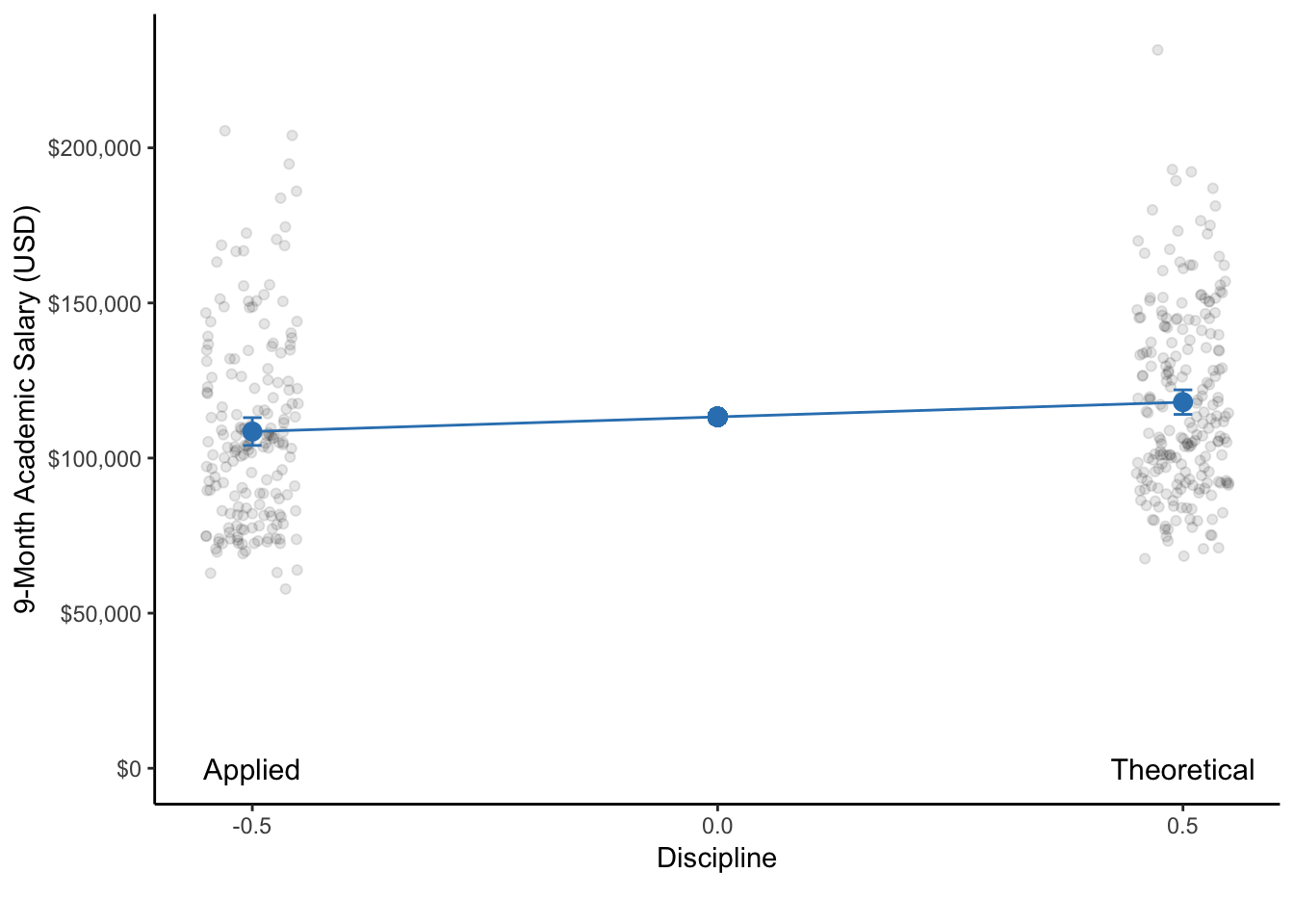

A dot plot of the 9-month academic salaries of professors that are in applied compared to theoretical disciplines. With respect to each discipline, the dot represents the mean salary and the bars represent the 95% CI.
Note: The data points of each group are actually only on a single line on the x-axis. They are only jittered (dispersed) for easier visualization of all data points.

Figure 9.1: A dot plot of the 9-month academic salaries of professors that are in applied compared to theoretical disciplines. With respect to each discipline, the dot represents the mean salary and the bars represent the 95% CI. Note: The data points of each group are actually only on a single line on the x-axis. They are only jittered (dispersed) for easier visualization of all data points.

\[b_1 = \frac{\Delta Y}{\Delta X} = \frac{\Delta Salary}{\Delta Discipline} = \frac{\Delta Salary}{1-0} = \frac{\Delta Salary}{1} = \Delta Salary\]↩
\[b_1 = \frac{\Delta Y}{\Delta X} = \frac{\Delta Salary}{\Delta Discipline} = \frac{\Delta Salary}{0-1} = \frac{\Delta Salary}{-1} = -\Delta Salary\]↩
\[b_1 = \frac{\Delta Y}{\Delta X} = \frac{\Delta Salary}{\Delta Discipline} = \frac{\Delta Salary}{0.5-(-0.5)} = \frac{\Delta Salary}{1} = \Delta Salary\]↩
\[b_1 = \frac{\Delta Y}{\Delta X} = \frac{\Delta Salary}{\Delta Discipline} = \frac{\Delta Salary}{1-(-1)} = \frac{\Delta Salary}{2}\]↩