Chapter 8 Dependent Samples t-Test

The dependent samples t-test is essentially the same analysis as the one sample t-test but on a difference score.

For example, let’s say that we were interested in determining if the weight of female patients with anorexia changed before the study compared to after the study.

For this example, we will be using the datasetAnorexia dataset.

We use a difference score because the measures of weight are dependent on (or relate to) each other as they come from the same individual. In other words, weights from the same individual are more likely to be closer in value than weights between individuals. If we do not take this dependence (i.e., positive dependence) into account, the t-value will be artificially inflated (or higher than it should be). Thus, we are also more likely to artificially reduce the p-value and ultimately commit a Type I error.

In other cases, not properly accounting for the dependence of measures can artificially reduce the t-value if the measures are negatively dependent. Measuring responsibility of household chores in couples is an example of negative dependence because as one couple rates their household chore responsbility as high or low, the other couple will typically rate the opposite. In other words, the measures of responsibility of household chores are more likely to be different within couples than the responsibility of household chores between couples. The artificially reduced t-value would increase the p-value and are ultimately likely to commit a Type II error.

8.1 Null and research hypotheses

8.1.1 Traditional approach

\[H_0: \mu_{WeightDifference} = 0\] \[H_1: \mu_{WeightDifference} \ne 0\]

The null hypothesis states that there is no weight difference in female patients with anorexia before and after the study. The research hypothesis states there is a weight difference in female patients with anorexia before and after the study.

8.1.2 GLM approach

\[Model: WeightDifference = \beta_0 + \varepsilon\] \[H_0: \beta_0 = 0\] \[H_1: \beta_0 \ne 0\]

where \(\beta_0\) represents the intercept and \(\varepsilon\) represents the error

Just like in the one sample t-test, the intercept (\(\beta_{0}\)) represents the sample mean. However, in this case, the sample mean is the mean of the weight difference of the female patients with anorexia before and after the study. Thus, the intercept here is testing if the sample mean of the weight difference score is significantly different than 0 with identical null and research hypotheses.

8.2 Statistical analysis

8.2.1 Traditional approach

To perform the traditional dependent samples t-test, we can again use the t.test() function. However, we will also set the paired option to TRUE.

t.test(datasetAnorexia$PostWeight, datasetAnorexia$PreWeight, paired = TRUE)

## 
##  Paired t-test
## 
## data:  datasetAnorexia$PostWeight and datasetAnorexia$PreWeight
## t = 2.9376, df = 71, p-value = 0.004458
## alternative hypothesis: true difference in means is not equal to 0
## 95 percent confidence interval:
##  0.8878354 4.6399424
## sample estimates:
## mean of the differences 
##                2.763889

From this output, we can see that the t-statistic (t) is 2.9376, degrees of freedom (df) is 71, and the p-value is 0.004458.

8.2.2 GLM approach

For the DV, we will input the difference of weight before and after treatment (i.e., PostWeight-PreWeight) directly into the lm() function. Since we are testing the intercept, we will again place 1 as the predictor.

model <- lm(PostWeight - PreWeight ~ 1, datasetAnorexia)

summary(model)

## 
## Call:
## lm(formula = PostWeight - PreWeight ~ 1, data = datasetAnorexia)
## 
## Residuals:
##     Min      1Q  Median      3Q     Max 
## -14.964  -4.989  -1.114   6.336  18.736 
## 
## Coefficients:
##             Estimate Std. Error t value Pr(>|t|)   
## (Intercept)   2.7639     0.9409   2.938  0.00446 **
## ---
## Signif. codes:  0 '***' 0.001 '**' 0.01 '*' 0.05 '.' 0.1 ' ' 1
## 
## Residual standard error: 7.984 on 71 degrees of freedom

Notice that in both analyses the sample mean difference of 2.76, the t-statistic of 2.94 with 71 degrees of freedom (df), and the p-value of .004 are identical with respective to place of rounding.

In this case, the systematic difference of the t-statistic is the difference in weight before and after a study and the unsystematic difference is standard error of the mean of the differences (in other words, random variability of the difference scores).

In this case, the probability of finding a t-statistic of 2.94 or more extreme is .004, which is very small and not likely to occur by chance if the null hypothesis was true.

8.3 Statistical decision

Given the p-value of 0.004 is smaller than the alpha level (\(\alpha\)) of 0.05, we will reject the null hypothesis.

8.4 APA statement

A dependent samples t-test was performed to test if female patients with anorexia had changed their weight before and after the study. The female patients with anorexia significantly gained weight after the study (M = 85, SD = 8) compared to before the study (M = 82, SD = 5), t(71) = 2.94, p = .004.

8.5 Visualization

# calculate descriptive statistics along with the 95% CI
dataset_summary <- datasetAnorexia %>%
  summarize(
    mean = mean(PostWeight - PreWeight),
    sd = sd(PostWeight - PreWeight),
    n = n(),
    sem = sd / sqrt(n),
    tcrit = abs(qt(0.05 / 2, df = n - 1)),
    ME = tcrit * sem,
    LL95CI = mean - ME,
    UL95CI = mean + ME
  )

ggplot(datasetAnorexia, aes("", PostWeight - PreWeight)) +
  geom_hline(yintercept = 0, alpha = .1, linetype = "dashed") +
  geom_jitter(alpha = 0.25, width = 0.02) +
  geom_errorbar(data = dataset_summary, aes(y = mean, ymin = LL95CI, ymax = UL95CI), width = 0.01, color = "#3182bd") +
  geom_point(data = dataset_summary, aes("", mean), size = 3, color = "#3182bd") +
  labs(x = 0, y = "Weight Difference (lbs)") +
  theme_classic()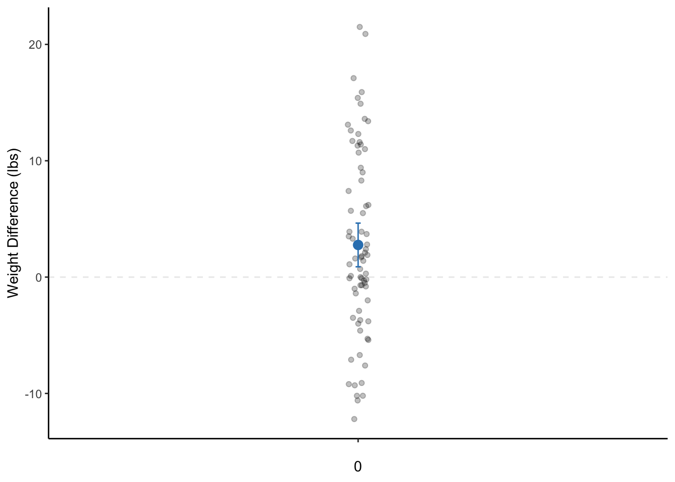

Figure 8.1: A dot plot of the weight change of female patients with anorexia before and after the study. The dot is the mean weight change and the bars represent the 95% CI. Note: The data points are actually only on a single line on the x-axis. They are only jittered (dispersed) for easier visualization of all data points.