Chapter 11 Factorial ANOVA
The factorial ANOVA, which tests more than one categorical IV, is an extension of the one-way ANOVA, which only tests one categorical IV. We can also think of the one-way ANOVA as a special case of the factorial ANOVA. In addition to testing the main effects of the categorical IV, the factorial ANOVA also tests the interactions of the categorical IVs.
For example, let’s say in addition to the question we asked in the independent samples t-test chapter (i.e., are salaries of professors different depending on their discipline?). Let’s also say that we were interested in two more questions:
- Does the salary of professors depend on their sex?
- Does the relationship between salary of professors and their discipline also depend on their sex?
The first question is the overall effect of a categorical IV, which is known as a main effect. The second question is the interaction of the two main effects (i.e., discipline and sex) and is automatically formed and tested in traditional factorial ANOVA.
(Note: Depending on our specific research questions, the interaction term may or not be needed. Thus, the automatic formation of the interaction within the traditional factorial ANOVA may not always be beneficial. Using the GLM approach gives us the flexibility to include or not include interaction terms.)
For this example, we will again use the datasetSalaries dataset.
Before we continue, let’s again check the contrasts of both variables.
contrasts(datasetSalaries$discipline)## Theoretical
## Applied 0
## Theoretical 1contrasts(datasetSalaries$sex)## Male
## Female 0
## Male 1Both of the variables are currently dummy coded.
Since we prefer a priori orthogonal contrast code, let’s go ahead and change the contrast for both of these factors.
We can code professors in the applied discipline as 0.5 and professors in the theoretical discipline as -0.5 since we think that those in the applied discipline will be earn a higher salary.
Similarly, we can code male professors as 0.5 and female professors as -0.5 since we also think that male professors will likely earn a higher salary than female professors.
Note: Since each factor is orthogonal within its respective factor, the sum of each contrast pair between the factors is also equal to 0. Thus, we do not need to actually check this; however, we encourage you test this on your own.
contrasts(datasetSalaries$discipline) <- cbind(AppliedvTheoretical = c(1 / 2, -1 / 2))contrasts(datasetSalaries$discipline)## AppliedvTheoretical
## Applied 0.5
## Theoretical -0.5contrasts(datasetSalaries$sex) <- cbind(FemalevMale = c(-1 / 2, 1 / 2))contrasts(datasetSalaries$sex)## FemalevMale
## Female -0.5
## Male 0.511.1 Null and research hypotheses
Given that there are a total of three questions of interest, there will also be three pairs of null and research hypotheses.
11.1.1 Traditional Approach
Main Effect of Discipline \[H_0: \mu_{Applied} = \mu_{Theoretical}\] \[H_1: \mu_{Applied} \ne \mu_{Theoretical}\]
The null hypothesis states that there is no difference in a professor’s salary whether they work in an applied discipline compared to a theoretical discipline on average across sex. The research hypothesis states that there is salary difference in professors in the applied discipline compared to the theoretical discipline on average across sex.Main Effect of Sex \[H_0: \mu_{Female} = \mu_{Male}\] \[H_1: \mu_{Female} \ne \mu_{Male}\]
The null hypothesis states there is no salary difference in professors that are female compared to those that are male on average across discipline. The research hypothesis states there is a salary difference in professors that are female compared to those that are male on average across discipline.Main Interaction Effect of Discipline by Sex \[H_0: \mu_{Female_{Applied}} - \mu_{Female_{Theoretical}} = \mu_{Male_{Applied}} - \mu_{Male_{Theoretical}}\] \[H_0: \mu_{Female_{Applied}} - \mu_{Female_{Theoretical}} \ne \mu_{Male_{Applied}} - \mu_{Male_{Theoretical}}\]
The null hypothesis states that the effect of discipline (i.e., the difference of theoretical and applied) are the same for males and females. In other words, the relationship between a professor’s salary and their discipline does not also change depending on their sex. The research hypothesis states that the relationship between a professor’s salary and their discipline does change based on their sex.
If we were interested in determining if the relationship between sex and salary depended on discipline, we could swap the subscripts so that sex is the subscript of discipline.
11.1.2 GLM Approach
\(Model: Salary = \beta_0 + \beta_1*Discipline + \beta_2*Sex + \beta_3*Discipline*Sex + \varepsilon\)
Main Effect of Discipline \[H_0: \beta_1 = 0\] \[H_1: \beta_1 \ne 0\]
The null hypothesis states that the slope associated with discipline is 0. Since the difference of our contrast is 1, the slope represents the mean salary difference between discipline on average across sex. In other words, the null hypothesis states that there is no difference in a professor’s salary based on their discipline on average across sex. The research hypothesis states that there is a difference in a professor’s salary based on their discipline on average across sex.Main Effect of Sex \[H_0: \beta_2 = 0\] \[H_1: \beta_2 \ne 0\]
The null hypothesis states that the slope associated with sex is 0. Since the difference of our contrast is 1, the slope represents the mean salary difference between sex on average across discipline. In other words, the null hypothesis states a professor’s salary is not related to their sex on average across their discipline. The research hypothesis states that a professor’s salary is related to their sex on average across their discipline.Main Interaction Effect of Discipline by Sex \[H_0: \beta_3 = 0\] \[H_1: \beta_3 \ne 0\]
The null hypothesis states that the slope associated with the interaction of discipline and sex is 0. Slopes associated with interactions can be thought of as changes in the slope associated with one IV included in the interaction for every 1 unit of another IV included in the interaction. In other words, if we calculated the slope between salary and discipline for just female professors and then calculated the slope between salary and discipline for just male professors, \(\beta_3\) represents the difference in these slopes. Since the difference of our contrast for sex is 1, the slope represents the difference in the slope between salary and discipline between males and females. The null hypothesis states that the relationship between a professor’s salary and their discipline does not change based on their sex. The research hypothesis states that the relationship between a professor’s salary and their discipline does change based on their sex.
11.2 Statistical analysis
11.2.1 Traditional approach
To perform a traditional factorial ANOVA, we can again use the aov() function. In the first argument, which is the formula, we can enter the DV followed by the tilde (~) and then the IVs along with its interaction. We can indicate an interaction by placing a colon (:) between the two IVs we want to interact. Specifically, this will create a new interaction term by multiplying the two IVs for each subject.
model <- aov(salary ~ discipline + sex + discipline:sex, datasetSalaries)We can also more concisely place an asterisk (*) between the two IVs to perform the exact same test (i.e., a test of an interaction along with a test for each main effect included in the interaction term). We prefer this form as we prefer simplicity.
model <- aov(salary ~ discipline * sex, datasetSalaries)Anova(model, type = c("III"))## Anova Table (Type III tests)
##
## Response: salary
## Sum Sq Df F value Pr(>F)
## (Intercept) 1.6139e+12 1 1834.2735 < 2.2e-16 ***
## discipline 7.9856e+09 1 9.0759 0.002758 **
## sex 7.4307e+09 1 8.4453 0.003867 **
## discipline:sex 1.7395e+09 1 1.9770 0.160492
## Residuals 3.4579e+11 393
## ---
## Signif. codes: 0 '***' 0.001 '**' 0.01 '*' 0.05 '.' 0.1 ' ' 1- Main Effect of Discipline
We can see from the F-statistic (F value) that the ability for discipline to explain salary is about 9.0759 times greater than its inability to explain salary, which is very large.
- Main Effect of Sex
We can also see that the ability for sex to explain salary is about 8.4453 times greater than its inability to explain salary, which is also very large.
- Interaction Effect of Discipline by Sex
However, the ability for the interaction between sex and discipline to explain salary is about 1.9770 times greater than its inability to explain salary, which is pretty small (close to 1).
11.2.2 GLM approach
model <- lm(salary ~ 1 + discipline * sex, datasetSalaries)Anova(model, type = c("III"))## Anova Table (Type III tests)
##
## Response: salary
## Sum Sq Df F value Pr(>F)
## (Intercept) 1.6139e+12 1 1834.2735 < 2.2e-16 ***
## discipline 7.9856e+09 1 9.0759 0.002758 **
## sex 7.4307e+09 1 8.4453 0.003867 **
## discipline:sex 1.7395e+09 1 1.9770 0.160492
## Residuals 3.4579e+11 393
## ---
## Signif. codes: 0 '***' 0.001 '**' 0.01 '*' 0.05 '.' 0.1 ' ' 1Note that in both analyses, the statistics are identical for each research question:
Main Effect of Discipline
When we look at the row for discipline, the F-statistic of5.41with1between degrees of freedom (df),393within degrees of freedom (df), and p-value of.020are identical.Main Effect of Sex
When we look at the row for sex, the F-statistic of1.22with1between degrees of freedom (df),393within degrees of freedom (df), and p-value of.270are identical.Main Interaction Effect of Discipline by Sex
When we look at the row for the interaction of discipline and sex (discipline:sex) the F-statistic of1.98with1between degrees of freedom (df),393within degrees of freedom (df), and p-value of.160are identical.
summary(model)##
## Call:
## lm(formula = salary ~ 1 + discipline * sex, data = datasetSalaries)
##
## Residuals:
## Min 1Q Median 3Q Max
## -52900 -23149 -5419 20505 112785
##
## Coefficients:
## Estimate Std. Error t value
## (Intercept) 107440 2509 42.828
## disciplineAppliedvTheoretical 15115 5017 3.013
## sexFemalevMale 14580 5017 2.906
## disciplineAppliedvTheoretical:sexFemalevMale -14109 10034 -1.406
## Pr(>|t|)
## (Intercept) < 2e-16 ***
## disciplineAppliedvTheoretical 0.00276 **
## sexFemalevMale 0.00387 **
## disciplineAppliedvTheoretical:sexFemalevMale 0.16049
## ---
## Signif. codes: 0 '***' 0.001 '**' 0.01 '*' 0.05 '.' 0.1 ' ' 1
##
## Residual standard error: 29660 on 393 degrees of freedom
## Multiple R-squared: 0.0482, Adjusted R-squared: 0.04094
## F-statistic: 6.634 on 3 and 393 DF, p-value: 0.0002217The estimates are slightly different now with the addition of another IV and its interaction, so we will interpret the estimate of each predictor.
The intercept (\(b_0\)) still represents the value of the DV when all IVs are 0. Since the codes of our categorical IVs are orthogonal (i.e., 0 lies in the middle of the categorical IV codes), the (Intercept) represents the 9-month academic salary of professors on average across discipline and sex. We don’t need to mention when the interaction is also 0 because if the two variables within the interaction are zero, then the interaction must also equal 0.
The estimate for the slope associated with discipline (\(b_1\)) represents the change in salary for every 1 unit increase in discipline when sex equals 0. Since the difference in the coding scheme of discipline is 1 and since 0 lies in-between the two codes for sex, the slope represents the mean salary difference of professors in applied compared to theoretical discipline on average across sex. Specifically, it is estimated that professors in the theoretical discipline earn $15,115 less than professors in an applied discipline on average across sex. We need to say on average across sex because we have an interaction term and are allowing for the slopes to vary at different levels of each IV.
The estimate for the slope associated with sex (\(b_2\)) is interpreted similarly to the slope associated with discipline. The estimate for the slope associated with sex represents the change in salary for every 1 unit increase in sex when discipline equals 0. Again, since the difference in the coding scheme for sex is 1 and since 0 lies in-between the two codes for discipline, the slope represents the mean salary difference of professors that are female compared to professors that are male on average across discipline. Specifically, it is estimated that professors that are male earn $14,580 more than professors that are female on average across discipline.
The estimate for the slope associated with the interaction of discipline and sex (\(b_3\)) represents the change in the slope of salary and discipline for every 1 unit increase in sex. Since the difference in the coding scheme of sex is 1, the slope represents the sex difference of the slope of salary and discipline. Specifically, the slope of salary and discipline is estimated to decrease by $14,109 for males compared to females In other words, the negative relationship between salary and discipline is expected to strengthen for males compared to females.
11.3 Statistical decision
Let’s examine the statistical decision for each research question.
Main Effect of Discipline
Given the p-value of.020is less than the alpha level (\(\alpha\)) of 0.05, we will reject the null hypothesis.Main Effect of Sex
Given the p-value of.270is greater than the alpha level (\(\alpha\)) of 0.05, we will retain (or fail to reject) the null hypothesis.Interaction Effect of Discipline by Sex
Given the p-value of.160is greater than the alpha level (\(\alpha\)) of 0.05, we will retain (or fail to reject) the null hypothesis.
11.4 APA statement
A factorial Analysis of Variance (ANOVA) was performed to test if 1) the salary of professors was different depending on their discipline, 2) the salary of professors was different depending on their sex, and 3) the relationship between salary of professors and their sex depending on their discipline. There was significant main effect of discipline on salary, F(1,393) = 9.08, p = .003. There was also a significant main effect of sex on salary, F(1,393) = 8.45, p = .004. However, the relationship between salary of professors and their sex did not change depending on their discipline, F(1,393) = 1.98, p = .160.
11.5 Visualization
# calculate descriptive statistics along with the 95% CI
dataset_summary <- datasetSalaries %>%
  group_by(discipline, sex) %>%
  summarize(
    mean = mean(salary),
    sd = sd(salary),
    n = n(),
    sem = sd / sqrt(n),
    tcrit = abs(qt(0.05 / 2, df = n - 1)),
    ME = tcrit * sem,
    LL95CI = mean - ME,
    UL95CI = mean + ME
  ) %>%
  mutate(discipline_code = ifelse(discipline == "Applied", 1 / 2, -1 / 2))

# plot
datasetSalaries %>%
  mutate(discipline_code = ifelse(discipline == "Applied", 1 / 2, -1 / 2)) %>%
  ggplot(., mapping = aes(discipline_code, salary, group = sex, shape = sex, color = sex)) +
  geom_jitter(alpha = 0.2, width = 0.2) +
  geom_point(
    data = dataset_summary, aes(x = discipline_code, y = mean),
    size = 3
  ) +
  geom_line(data = dataset_summary, aes(x = discipline_code, y = mean)) +
  geom_errorbar(
    data = dataset_summary, aes(x = discipline_code, y = mean, ymin = LL95CI, ymax = UL95CI),
    width = 0.02
  ) +
  labs(
    x = "Discipline",
    y = "9-Month Academic Salary (USD)",
    color = "Sex",
    shape = "Sex"
  ) +
  theme_classic() +
  scale_x_continuous(breaks = seq(-2, 2, 1 / 2), limits = c(-1, 1)) +
  scale_y_continuous(labels = scales::dollar) +
  annotate(geom = "text", x = -.5, y = 0, label = "Applied", size = 4) +
  annotate(geom = "text", x = .5, y = 0, label = "Theoretical", size = 4)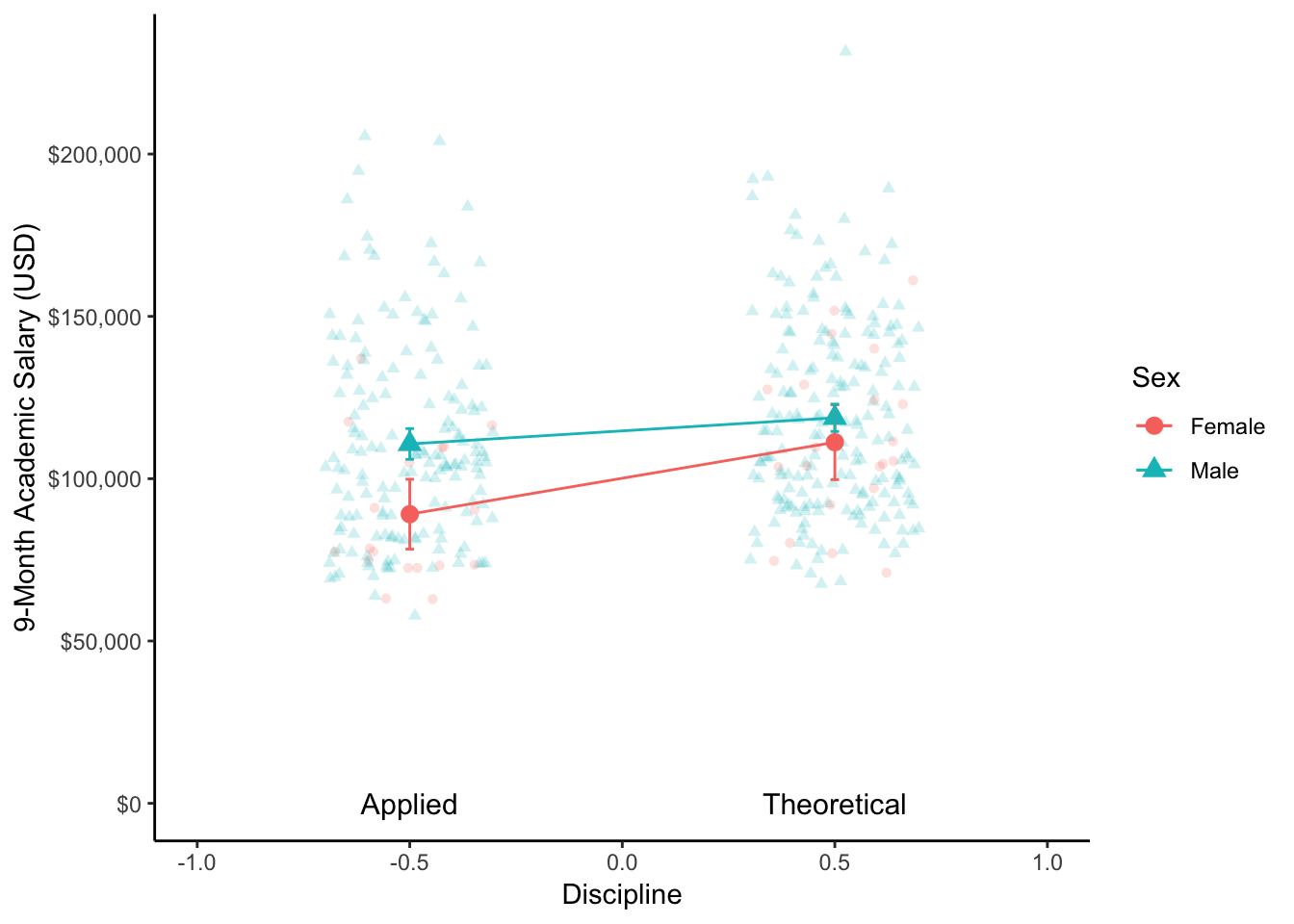
Figure 11.1: A dot plot of the 9-months salaries of professors by their discipline and sex. Respectively for each discipline and sex, the dot represents the mean and the bars represent the 95% CI.