Chapter 6 Correlation

The next analysis that we will go over is the correlation. The correlation and simple linear regression are similar with the only difference being that the estimate of the slope of the correlation is standardized, while the estimate of the slope of the simple linear regression is unstandardized.

The correlation that is typically taught is the Pearson correlation, which is the correlation between two continuous variables. However, despite the difference in correlation nomenclature for different variable types, these correlations are similarly applied in the GLM approach.

As a side note, this is also the chapter that people associate the phrase “correlation is not causation.” This phrase is correct and should be thoughtfully considered. All statistical analyses are looking at how variables relate (or correlate or covary) with each other. Thus, the phrase “correlation is not causation” is about research design rather than statistical analysis.

Given that the simple linear regression and correlation are similar, we can use the same example from the previous chapter, where we were interested in determining if there was a relationship (or correlation) between the number of years since a professor has had their Ph.D. and their salary. We will be using the same datasetSalaries dataset to facilitate comparisons.

6.1 Null and research hypotheses

6.1.1 Traditional approach

\[H_0: \rho = 0\] \[H_1: \rho \ne 0\]

where $\rho$ represents the population correlation value (Note: $r$ represents the estimated population correlation value or sample correlation value.)

The null hypothesis states that there is no correlation between the amount of years since earning a Ph.D. and their salary (i.e., their relationship is equal to 0). In contrast, the research hypothesis states there is a correlation (i.e., the relationship is not equal to 0).

6.1.2 GLM approach

\[Model: Z_{salary} = \beta_0 + \beta_1*Z_{years.since.phd} + \varepsilon\] \[H_0: \beta_1 = 0\] \[H_1: \beta_1 \ne 0\]

where Z is the standardized (i.e., z-scored) version of that particular variable. As a reminder, z-scoring converts a variable to have a mean of 0 and a standard deviation of 1, but its distribution is unchanged.

In this example, the correlation value ($r$) is simply a standardized slope ($\beta$). Thus, standardizing both the DV and IV standardizes the slope. In other words, $r$ is the standardized form of $b$. (Note: The estimated standardized slope within the regression context is unfortunately referred to by the same symbol as the true population regression coefficient symbol, $\beta$.)

6.2 Statistical analysis

6.2.1 Traditional approach

Using the traditional approach, we can test the correlation by using the cor.test() function. The first input is the IV (yrs.since.phd) and the second input is the DV (salary). However, the order is essentially arbitrary and can be switched. Notice that in each input, we also included the name of the dataset (i.e., datasetSalaries) before each variable, which is seperated by a $. The $ calls an object within a larger object. In this case, the $ calls the object or variable yrs.since.phd within the larger object of the datasetSalaries dataset.

cor.test(datasetSalaries$yrs.since.phd, datasetSalaries$salary)

## 
##  Pearson's product-moment correlation
## 
## data:  datasetSalaries$yrs.since.phd and datasetSalaries$salary
## t = 9.1775, df = 395, p-value < 2.2e-16
## alternative hypothesis: true correlation is not equal to 0
## 95 percent confidence interval:
##  0.3346160 0.4971402
## sample estimates:
##       cor 
## 0.4192311

The new statistic that is shown in this analysis is the correlation (cor) and the 95 percent confidence interval. The correlation is the estimated correlation, $r$, which equals 0.42. The 95% confidence interval represents our probabilistic confidence (i.e., 95% confident) that our true population correlation, $\rho$, would fall between the values of 0.33 and 0.50.

6.2.2 GLM approach

To perform a correlation using the GLM approach, we can again use the lm function.

model <- lm(scale(salary) ~ 1 + scale(yrs.since.phd), data = datasetSalaries)

Remember, both the DV and IV need to be standardized so that our estimates are also standardized. Luckily, we can standardize both salary and yrs.since.phd directly in the formula by using the scale function.

The table that most aligns with the correlation output is the coefficients table and not the ANOVA source table, so we will only be using the summary() function for this analysis. However, we could use the Anova() function to obtain the ANOVA source table if desired.

summary(model)

## 
## Call:
## lm(formula = scale(salary) ~ 1 + scale(yrs.since.phd), data = datasetSalaries)
## 
## Residuals:
##     Min      1Q  Median      3Q     Max 
## -2.7789 -0.6415 -0.0944  0.5311  3.3802 
## 
## Coefficients:
##                        Estimate Std. Error t value Pr(>|t|)    
## (Intercept)          -5.886e-17  4.562e-02   0.000        1    
## scale(yrs.since.phd)  4.192e-01  4.568e-02   9.177   <2e-16 ***
## ---
## Signif. codes:  0 '***' 0.001 '**' 0.01 '*' 0.05 '.' 0.1 ' ' 1
## 
## Residual standard error: 0.909 on 395 degrees of freedom
## Multiple R-squared:  0.1758, Adjusted R-squared:  0.1737 
## F-statistic: 84.23 on 1 and 395 DF,  p-value: < 2.2e-16

Since the estimates are standardized, the units are in standard deviations rather than their original metric.

For example, the slope represents the standard deviation unit change in Y (scale(yrs.since.phd)) for every one standard deviation unit increase in X (salary). In other words, there is a 0.42 standard deviation unit increase in salary for every one standard deviation unit increase in the number of years a professor has had their Ph.D.

The intercept represents Y (salary) in standard deviation units when X (yrs.since.phd) is 0 standard deviation units, or at the average value of X (yrs.since.phd). Remember, that 0 standard deviations (or a z-score of 0) is also the mean because z-scoring converts the mean to 0 and the standard deviation to 1. In other words, for a professor that has had their Ph.D. for 0 standard deviation units (or an average number of years), their predicted salary is -5.89e-17 standard deviation units.

Given these interpretations of standardized slopes and intercepts, they are not our preference, especially when variables have easily interpreted metrics. However, standardized slopes and intercepts are preferred for quickly determining effect sizes as they can only range between -1 and +1. They are also preferred when comparing other predictors within and between other models as they are in a standardized metric; however, the validity of these comparisons are debated.

confint(model)

##                            2.5 %     97.5 %
## (Intercept)          -0.08969389 0.08969389
## scale(yrs.since.phd)  0.32942404 0.50903818

Notice that in both analyses the values are identical with respect to place of rounding. The correlation $r$ value is .42, t-statistic is 9.18 with 395 degrees of freedom (df), and the p-value is 2.2e-16.

6.3 Statistical decision

Given the p-value of 2.2e-16 is smaller than the alpha level ($\alpha$) of 0.05, we will reject the null hypothesis.

6.4 APA statement

A correlation was performed to test whether the amount years since obtaining a Ph.D. is related to salary. The amount of years since obtaining a Ph.D. was significantly related to salary, r(395) = 0.42, p < .001.

6.5 Visualization

ggplot(datasetSalaries, aes(scale(yrs.since.phd), scale(salary))) +
  geom_point(alpha = 0.25) +
  geom_smooth(method = "lm", color = "#3182bd") +
  labs(
    x = "Years since Ph.D.",
    y = "9-Month Salary (USD)"
  ) +
  scale_y_continuous(labels = dollar) +
  theme_classic()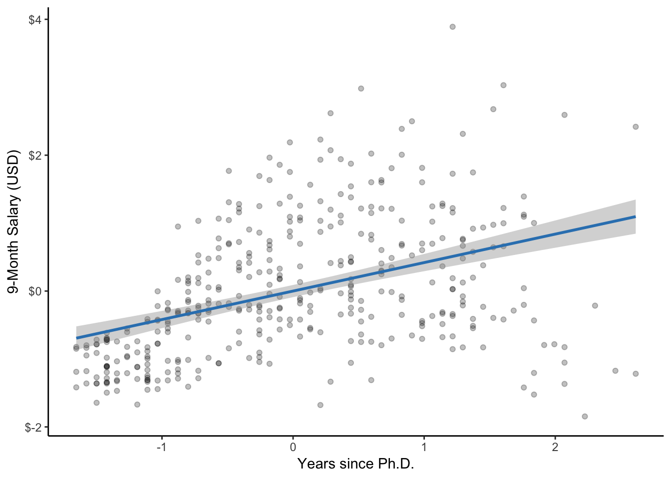

Figure 6.1: A scatterplot of years since Ph.D. and salary along with the line of best fit. The gray band represents the 95% CI.