
Module 3: Disease Mapping: Spatial Empirical Bayes
Additional Resources
- Anselin, L. Spatial Regression Analysis in R: A workbook. 2007.
- GeoDa Center Resources: Section on distance-based spatial weights
- GeoDa Center Resources: Section on contiguity-based spatial weights
Spatial Thinking in Epidemiology
- This is the first time where we will formally incorporate and make explicit what spatial means in spatial analysis.
- Although all work up until now has been represented on a map (thus spatially contextualized), we have not formally incorporate spatial relationships into any aspect of analysis.
- Empirical Bayes Estimators treat each spatial unit as if it were spatially or geographically independent of every other spatial unit.
- This assumption that units are geographically independent is what I have referred to as aspatial analysis.
An argument for the relevance of space
- The fundamental dimension for spatial relations in geography is that of distance (and relatedly the idea of proximity), whether that be euclidean (e.g. as the crow flies) distance, social distance, or network distance.
- Based on Tobler’s First Law of Geography, near things tend to be more alike (e.g. correlated although not necessarily causally linked) than distant things (on average), implying a kind of dependence or correlation among local units that might not be evident overall.
- We can ‘borrow’ statistical information from spatial neighbors to supplement estimation of local disease parameters.
- This is exactly what we will do with spatial Empirical Bayes estimation, where instead of using the overall (global) rate of disease as the prior, we will use the local rate for neighbors surrounding each entity as a kind of custom, place-specific prior.
The table below illustrates we can define which units are near which other units using different definitions, and those definitions have slightly different assumptions and results.
Below is a brief summary of several common neighbor definitions:
| Basic metric | Description | |
|---|---|---|
| Rook | Contiguity | Unit A and unit B are neighbors if and only if they share boundary edges. Second or higher-order contiguity refers to units sharing edges with index unit (1st order contiguity), plus units that share boundary edges with all 1st order neighbors; and so forth) |
| Queen | Contiguity | Unit A and unit B are neighbors if they share either boundary edges or boundary corners (e.g. vertices). Second or higher-order contiguity refers to units sharing edges with index unit (1st order contiguity), plus units that share boundary edges with all 1st order neighbors; and so forth) |
| Sphere of influence graph neighbors | Contiguity | Graph-based neighbors start by creating Delauney triangles from the centroid of units. Neighbors are defined by the edges of the triangles. |
| Fixed distance | Distance | Unit A is a neighbor of unit B, if unit A (or perhaps the centroid of the unit) falls within a fixed-distance buffer created around unit B (or perhaps the centroid of the unit). |
| K-nearest neighbors (KNN) | Distance | Unit A is a neighbor of unit B, if when a rank-order of closest to furthest neighbors from Unit B is created, Unit A is ranked \(\leq k\). In other words, if \(K\) is set to 5, then unit A is neighbor of B if it is among the 5 nearest neighbors. KNN is an asymmetric definition; it is possible for A to be neighbors with B, but B may not be a neighbor to A. |
| Inverse distance | Distance | Instead of using a fixed threshold of distance (e.g. a buffer) or a fixed number of near neighbors (e.g. KNN), this strategy describes proximity or ‘nearness’ as the inverse of the Euclidean or road-network distance (or possibly inverse of distance-squared). |
The choice of which neighbor definition to use is influenced by several study-specific factors, some of which can be in conflict with others:
- Variation in size of areal units across the study area. If some areal units are very small (e.g. counties in the Eastern U.S.) and some are very large (e.g. counties in the Western U.S.), then the geographic area defined by adjacent counties will be quite different (e.g. think about how long it takes to drive across two counties like Dekalb and Fulton in Atlanta, versus how long it might take to traverse two counties in Nevada or Utah). In contrast, fixed-distance neighbors will have a more consistent among of linear distance between index units and their neighbors.
- Assumptions or requirements of the statistical analysis of interest. Some algorithms require/expect features such as neighbor symmetry or spatial weights row standardization to account for unequal numbers of neighbors.
- The assumed meaning of space in the analysis. It is possible that, for instance, the meaning of distance in Western counties is different where further travel to basic services is more the norm than in denser areas in the East.
- The purpose and audience of the map. It is important to make the analysis accessible and interpretable to the target audience.
- Aspects of the geography including islands or presence of non-contiguous units (e.g. Hawaii, Alaska, Puerto Rico)
Spatial Analysis in Epidemiology
To apply these concepts to specific spatial analysis, we will continue to use the Georgia opioid mortality dataset used in the previous module of the eBook. As a reminder, this is a county-level dataset for the \(n=159\) Georgia Counties containing the count and rate of opioid related deaths. Moving forward we will use Queen’s Contiguity where neighbors are defined if there is a shared boundary between counties.
Creating contiguity neighbor objects
In R, the spdep package has a series of functions useful for creating spatial weights matrices. In general, the process of going from a spatial object (e.g. an sf class data object) to a usable spatial weights matrix requires more than one step, and the steps vary depending on the eventual use.
Since we are starting with areal (polygon) data, the starting point is to use a utility function, poly2nb(), that take a polygon spatial object (of class sf or sp) and determine which specific polygon regions are contiguous with (touch, share boundaries with) other regions. If you review the help documentation, you will see that the function takes a spatial sf object as the input, with arguments specifying whether to use Queen contiguity (default; Rook is the alternative). The function returns something called a neighbor list.
# load the package spdep
library(spdep)

# Create a queen contiguity neighbor list
queen_nb <- poly2nb(data, queen = TRUE)

# Examine the resulting object
summary(queen_nb)
Neighbour list object:
Number of regions: 159
Number of nonzero links: 860
Percentage nonzero weights: 3.401764
Average number of links: 5.408805
Link number distribution:
1 2 3 4 5 6 7 8 9 10
1 4 12 29 36 37 28 9 1 2
1 least connected region:
41 with 1 link
2 most connected regions:
53 60 with 10 linksThe
summary()function fornbobjects (neighbor objects inspdep) provides high-level info, such as regions with no neighbors and the distribution of neighbors.Use
str(queen_nb)orqueen_nb[[1]]to inspect the structure or neighbors of the first region, sincenbobjects are lists where each element corresponds to a region’s neighbors.Neighbor objects are lists, with each element representing a region and its neighboring regions, ordered by the input dataset.
Spatial symmetry means if one region is a neighbor to another, the reverse is also true. This holds for contiguity-based neighbors (shared boundaries).
Visualizing neighbor connections can help understand the spatial relationship patterns and density when selecting a neighbor definition.
The
plot.nb()function requires thenbobject and a matrix of centroids to visualize neighbor links.
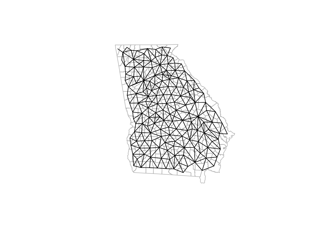
Notice how the density of neighbors is generally lower on the coast and at state boundaries. This systematic difference in neighbors can produce patterns sometimes referred to as edge effects. These edge effects could be a source of bias, because counties in the interior of the state have more neighbors (and thus more ‘local information’ on average) than border counties.
From spatial neighbors to spatial Disease Mapping
Summary of Empirical Bayes
We saw in the last module Empirical Bayes disease rate smoothing is a process by which we take a set of regions, and consider each of them as data, with the question,
‘What is the truest underlying rate of disease in this place?’
We compare these observed data with some prior belief or expectation of what the rate could plausibly be (not specifically, but approximately or within a range).
Aspatial Empirical Bayes smoothing we used the overall average rate for the entire study region (e.g. state of Georgia) as the prior. i.e., we sum all of the cases across spatial units (e.g. counties), and all of the population at risk across those units, to calculate a single reference rate, and the variance around that expectation.
Spatial Empirical Bayes
By using our newly-created definitions of local neighbors among Georgia counties we can extend the Empirical Bayes approach by changing the source of the prior information.
Instead of a global reference risk we can use the average of one’s neighbors as a prior.
This produces a sort of borrowing of statistical information through space, under the assumption that the local counties tell us more about a specific place than do counties far away.
This assumes the average the local information is more informative than non-local (global) prior information.
The function for estimating spatial Empirical Bayes is EBlocal() from the spdep package, and it requires not only the count of events and the count of population at risk for each county, but also a nb neighbor object. Although we highlighted the importance of neighbor symmetry above for some spatial analysis, symmetric neighbors are not required for spatial Empirical Bayes estimation.
eBayes (SpatialEpi) smooths based on global trends across the entire study area.
EBlocal (spdep) smooths based on local trends among neighboring regions, offering more spatial specificity.
Reference: Marshall R M (1991) Mapping disease and mortality rates using Empirical Bayes Estimators, Applied Statistics, 40, 283–294; Bailey T, Gatrell A (1995) Interactive Spatial Data Analysis, Harlow: Longman, pp. 303–306.
library(SpatialEpi)
library(spdep)

#Global Empirical Bayes
global_eb1 <- eBayes(data$death_count, data$expect)
data$ebSMR <- global_eb1$RR

# Estimate spatial (local) EB under the Queen contiguity neighbor definition
eb_queen <- EBlocal(data$death_count, data$pop_count, nb = queen_nb)

# The output fro EBlocal() is a 2 column data.frame. The second colum is the EB estimate
data$EB_queen <- eb_queen[,2]*10000 #Calculate the SMR
NOTE: there is currently no function in R to estimate spatial EB rates with credible/confidence intervals or p-values, as we could with the Poisson-Gamma model for aspatial. Fully Bayesian disease mapping (e.g. in Disease Mapping IV) would be the best approach if spatial methods producing credible/confidence intervals are desired.
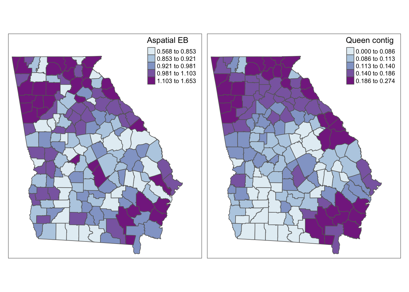
Visualizing alternate smoothing approaches
Here is some code for simple visual comparison of the raw/observed, aspatial EB, and a variety of spatially-smoothed EB estimates. As you review these maps, you might ask yourself the following questions:
- Where does any EB smoothing versus the raw/observed estimates differ?
- Where do the spatial EB estimates differ from the aspatial EB estimate?
- And what differences do you notice among the various spatial EB estimates, distinguished by their unique definitions of local?
Final thoughts: Making choices
We have quickly amassed a large number of analytic tools to address one problem in spatial epidemiology: reliably characterize spatial heterogeneity in the presence of rate instability and uncertainty due to data sparsity.
These analytic strategies include the two approaches to Empirical Bayes smoothing, but also the myriad of neighbor definitions for when we do choose a spatial approach.
Unfortunately there is no simple rule!
Below is a summary of considerations.
As with many things in epidemiologic analysis, there is an important role for science but also a need for experts who can engage in the art of analysis.
| Method | Uses | Assumptions and comments |
|---|---|---|
| Aspatial Empirical Bayes | Smooth or shrink local rates towards global (overall) reference rate, with shrinkage inversely proportionate to variance / sample size in local region. In one simulation study, aspatial (versus spatial) EB minimized mean-squared error (MSE) when the outcome is rare. |
1. The best prior estimation of plausible rates (mean and variance) is the overall average. 2. The reason for sparsity is about both numerator and denominator (e.g. both a rare disease, and small populations at risk). |
| Spatial Empirical Bayes | Smooth or shrink local rates towards local reference. In simulation study, spatial (local) EB outperformed aspatial when outcomes were not rare. | 1. There is at least some spatial auto correlation in rates such that nearby-regions rates serve as a more informative prior than the global average. 2. The reason for sparsity is primarily about the denominator (e.g. small population at risk), but the health outcome itself is not rare (in the overall region). |