Module 4: Spatial Mapping in R

Learning objectives by module
After this module you should be able to…
Perform basic coding operations in R
Produce simple thematic maps of epidemiologic data in R.

Additional Resources

sf cheatsheet

sf introduction

Geocomputation with R by Robin Lovelace. This will be a recurring ‘additional resource’ as it provides lots of useful insight and strategy for working with spatial data in R. I encourage you to browse it quickly now, but return often when you have questions about how to handle geographic data (especially of class sf) in R.

An introduction to the ggplot2 package. This is just one of dozens of great online resources introducing the grammar of graphics approach to plotting in R.

A basic introduction to the tmap package This is also only one of many introductions to the tmap mapping package. tmap builds on the grammar of graphics philosophy of ggplot2, but brings a lot of tools useful for thematic mapping!

Introduction to TIDYCENSUS

The tidycensus package by Kyle Walker is an R package designed to facilitate the process of acquiring and working with US Census Bureau (USCB) population data in the R environment.

It is designed to streamline the data wrangling process for spatial Census data analysis.

With tidycensus R users can acquire census reported variables of interest AND geometric and spatial attributes which helps facilitate mapping and spatial analysis.

US Census Bureau data consists of:

US decennial census data from 2010 and 2020 requested using \(get\_decennial()\).
1-year and 5-year American Community Survey (ACS) population and demographic data requested using \(get\_acs()\).
Population Projection Estimates (PEP) requested using \(get\_estimates()\).
ACS Public Use Microdata requested using \(get\_pums()\).
ACS Migration Flows requested using \(get\_flows()\).

Note this is not a comprehensive tutorial on tidycensus.

It will give you an introduction to the capabilities of the package.

For more information on USCB data products visit https://www.census.gov/data.html.

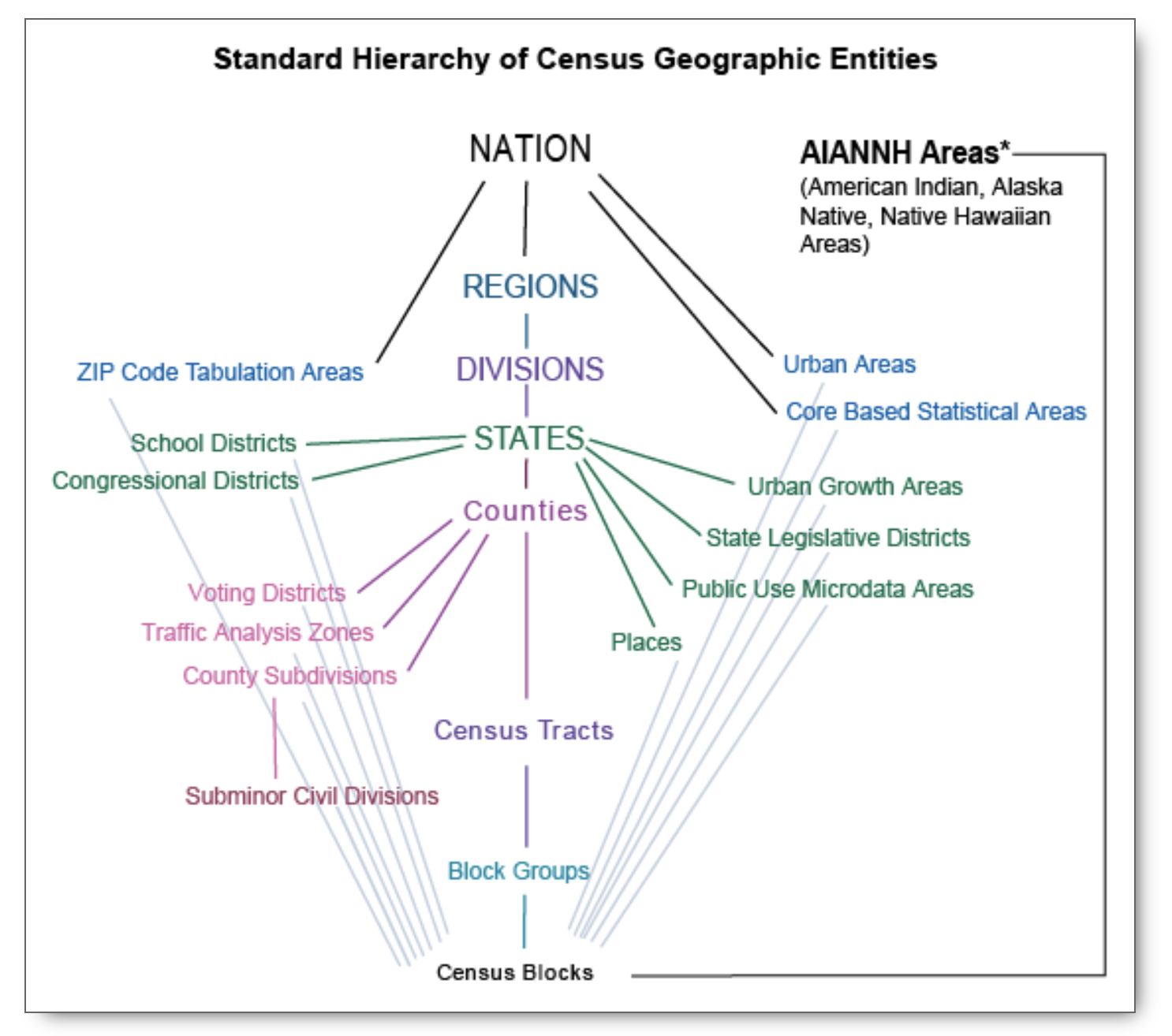
Geography in Tidycensus

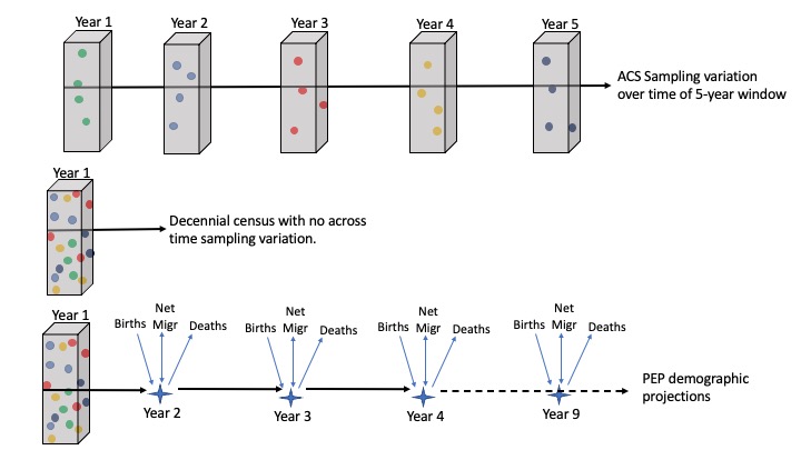
The USCB reports data from the national level to county to census block level.

Importantly, not all data sources report data at all geographies.

The decennial census and 5-year ACS estimates report down to census block.

However, PEP only reports down to county level and metro/micro-politan areas.

Searching for variables in Tidycensus

One challenge is extracting variable names from the USCB data sources.

The tidycensus package contains a \(load\_variable()\) function that can list variable names and their descriptions.

By browsing or subsetting the table, you can search for the relevant variables needed for your analysis.

# install.packages("tidycensus")

library(tidycensus)

#Read in ACS variables

vars <- load_variables(2020, "acs5")

head(vars)

Extracting the data in Tidycensus

Let’s work through examples on how to extract ACS.

The parameters passed through the \(get\_acs()\) function require the:

geography which the the spatial resolution you want reported.

Here we want county level data.

state is an optional parameter if you want a specific state.

The default is NULL if you want the US.

variables listed the needed variables from the list above.

Here we chose the variable for median household income.

year (self-explanatory?) 5.
geometry is an important parameter. When set to \(T\) the data frame will include the spatial boundaries of the counties in your data frame and will produce an \(sf\) object.

#Extract ACS median household income at county level for GA. 2020

ga_hinc <- get_acs(
  geography = "county",
  state = "Georgia",
  variables= c("B19013_001"),
  year = 2020,
  geometry = T)

head(ga_hinc)

The resulting data frame a row for each county.

Each row lists the county name, the estimate of the variable, and the associated margins of error (otherwise referred to as sampling error from ACS).

Additionally, we have a geographic identification (GEOID) and the geometric features column.

Next let’s work through examples on how to extract PEP.

The parameters passed through the \(get\_estimate()\) function require the:

geography which the the spatial resolution you want reported. Here we want county level data.
state is an optional parameter if you want a specific state. The default is NULL if you want the US.
product lists three optioins: (1) population totals (“population”), (2) populations by characteristics (“characteristics”), and (3) housing units (“housing”). Here we request populations by sex and race breakdowns.
**breakdown* lists RACE, SEX, AGE (for years 2020+), and HISPANIC.
year (self-explanatory?)
geometry again set to \(T\) the data frame will include the spatial boundaries of the counties in your data frame and will produce an \(sf\) object.

#Extract PEP populations by Race-Sex at county level for GA. 2019

ga_sexrace <- get_estimates(
  geography = "county",
  state = "Georgia",
  product= c("characteristics"),
  breakdown = c("SEX","RACE"),
  breakdown_labels = T,
  year = 2019,
  geometry = T)

head(ga_sexrace)

The resulting data frame a row for each county.

Each row lists the county name, the value of the variable.

For example, the population estimate for 2019 for the White population in Fulton County is 483838 across both sexes.

To map population data from the US Census Bureau, you must register a Census API key first. To obtain a census API go to https://api.census.gov/data/key_signup.html.

The in R type census_api_key(“YOUR KEY”, install = TRUE) to install the census API key. You only need to do this once.

From tidycensus you can extract information from the decennial census, Population Estimation Projection (PEP), and American Community Survey (ACS). Let’s see some examples:

First you may need to look up which variables to download from the data set: For example, we can look up all the listed variables in the ACS and find which variables have label “Cherokee”.

# Load variables for the 2020 Census decennial data
vars <- load_variables(year = 2020, dataset = "acs5", cache = TRUE)
head(vars)

name	label	concept	geography
B01001_001	Estimate!!Total:	SEX BY AGE	block group
B01001_002	Estimate!!Total:!!Male:	SEX BY AGE	block group
B01001_003	Estimate!!Total:!!Male:!!Under 5 years	SEX BY AGE	block group
B01001_004	Estimate!!Total:!!Male:!!5 to 9 years	SEX BY AGE	block group
B01001_005	Estimate!!Total:!!Male:!!10 to 14 years	SEX BY AGE	block group
B01001_006	Estimate!!Total:!!Male:!!15 to 17 years	SEX BY AGE	block group

This code extracts PEP population counts at the county level for Oklahoma.

#Extract county level population counts 
ok_population <- get_estimates(
  geography = "county",
  state = "Oklahoma",
  product= c("population"),
  year = 2022,
  geometry = T)

This code extracts PEP population counts by demographic breakdowns at the county level for Oklahoma. The PEP reported breakdowns are not available for recent years via tidycensus, and must be downloaded directly from USCB.gov.

#Extract county level population counts by characteristics
ok_characteristics <- get_estimates(
  geography = "county",
  state = "Oklahoma",
  product= c("characteristics"),
  breakdown = c("RACE", "SEX"),
  breakdown_labels = T,
  year = 2019, 
  geometry = T)

This code extracts ACS reported Cherokee population estimates at county level for Oklahoma.

ok_cherokee <- get_acs(
  geography = "county",
  state  = "Oklahoma",
  variables = "B02014_009",
  year = 2022,
  geometry=T
)

Introduction to Shapefile and Tigris

Shapefiles are a popular method of representing geospatial vector data in GIS.

The shapefile can store data in the form of points, lines, or polygons.

They can be used to represent administrative boundaries (think country/state/county borders) or roads, rivers, lakes etc.

These shapes, together with data attributes that are linked to each shape, create the representation of the geographic data.

Three mandatory files related to shapefiles use the extensions (.shp, .shx, .dbf).

The actual shapefile relates to the.shp file.

Shapefiles can be found on the internet with various publishers.

For example,the US census bureau publishes shapefiles for the entire US.

The USCB’s TIGER/Line database includes high-quality series of geographic datasets suitable for spatial and cartographic analyses.

The TIGER/Line shapefiles include three general types of data:

Legal entities: Legal geographic entities including county and state boundaries.
Statistical entities: Non legal entities but boundaries with statistical meaning, i.e., census tracts and. block groups.
Geographic features: Geographic datasets linked with aggregrate demographic information including water and road fetures.

From the USCB website, we downloaded the shapefile that contains all roads for the state of GA.

Using the \(sf\) package, we read in the shapefile using the \(st\_read\) function.

This gives an \(sf\) data frame that contains the geometric features from the shapefile.

Using the \(tmap\) package, we can plot the \(sf\) object.

library(sf)
#Read in a shapefile

shp <- st_read("data/shapefiles/tl_2019_13_prisecroads.shp")

class(shp)

head(shp)

#Plot boundaries contained in shapefile.

tm_shape(shp) +
  tm_lines(col = "black")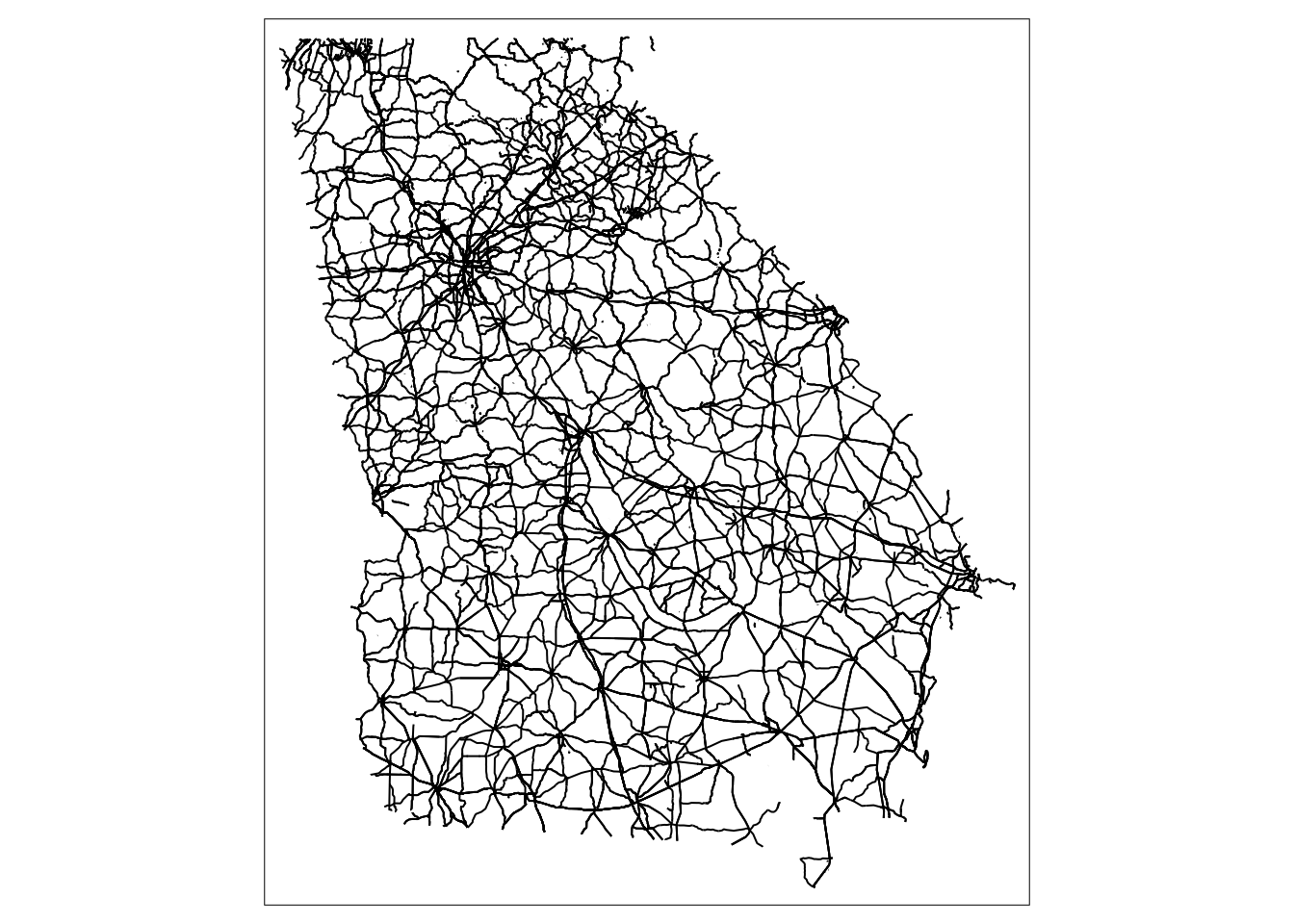

The tigris package simplifies the process for R users of obtaining and using Census geographic datasets.

The full list of shapefiles in tigris are available here

For example, the \(states()\) function can be used to download the boundaries of U.S. states.

This function produces an \(sf\) data frame with geometric features.

# install.pakcages("tigris", dep =T)

library(tigris)
library(tmap)

#Call in state boundaries for US

st <- states()
head(st)

Additionally, we can extract shapefiles corresponding to specific counties within a state.

library(tigris)
library(tmap)
#Extract county borders for GA from the tigris package

ga_counties <- counties("GA")

#Plot the county borders
tm_shape(ga_counties) +
  tm_borders(col = "black")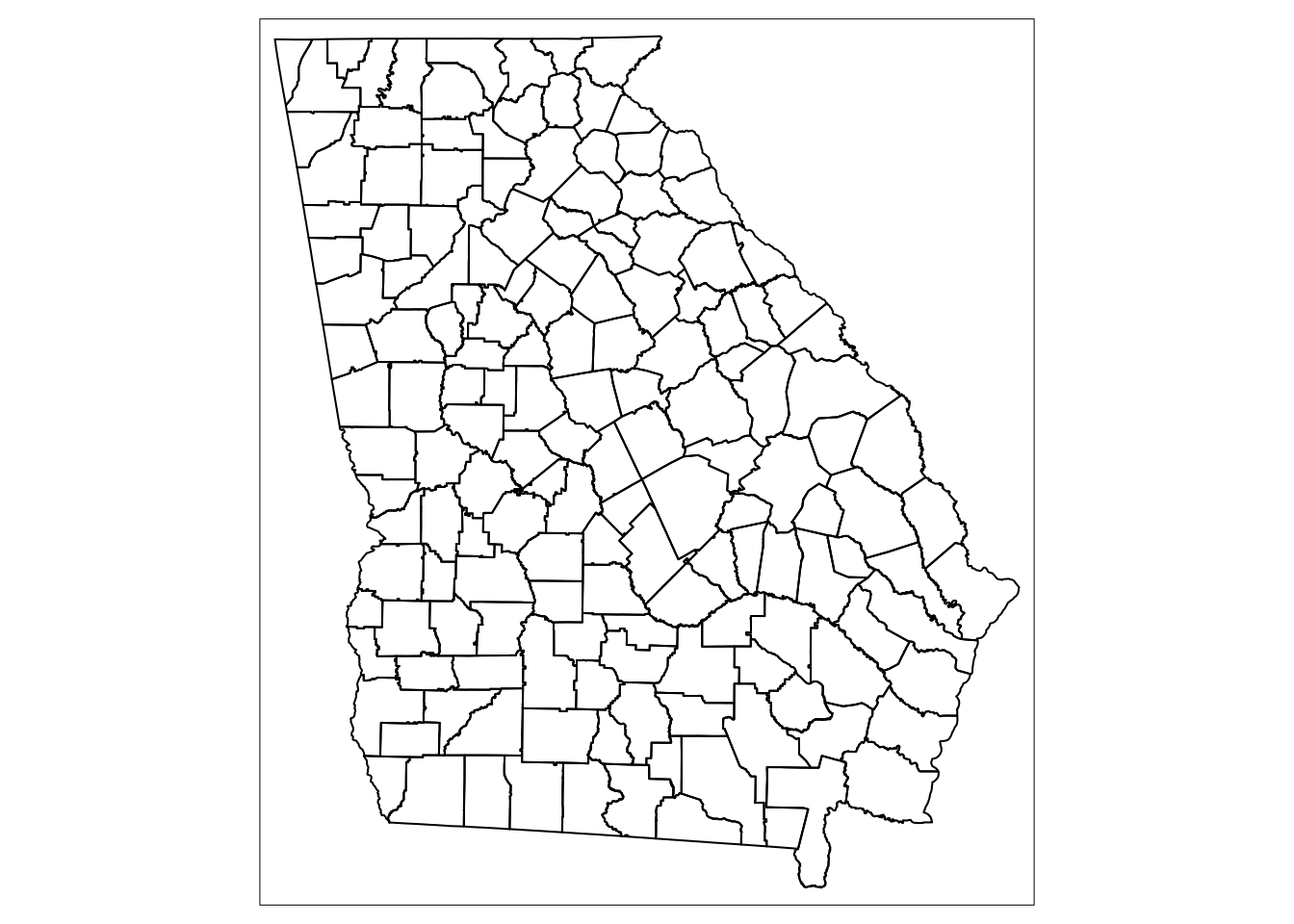

Let’s add to this map by adding roads and water areas.

We get the roads for GA using the \(primary\_secondary\_roads()\) function that requires the state parameter to be set.

To obtain the water areas, we must obtain water geometries for each county within the state of GA.

We use the \(area\_water()\) function that has state and county parameters.

#Extract the FIPS identifier for each county in GA

fips <- unique(ga_counties$COUNTYFP)

#Extract the primary and secondary roads for GA

road_data <- primary_secondary_roads("GA")

#To create areas of water, we must extract for each FIPS ID separately.

#Create a blank list

water_list <- list()

#For each county c, extract the water area using area_water()

#This takes a while!!!

for(c in 1:length(fips)){
water_list[[c]] <- area_water("GA", fips[c])
}

#Use the do.call and rbind functions to compile the list into a data frame

water_data <- do.call("rbind", water_list)

#Map the county borders, areas of water, and roads.

tm_shape(ga_counties) +
  tm_borders(col = "black") +
  tm_shape(water_data) +
  tm_borders(col = "blue") +
  tm_shape(road_data) +
  tm_lines(col = "orange")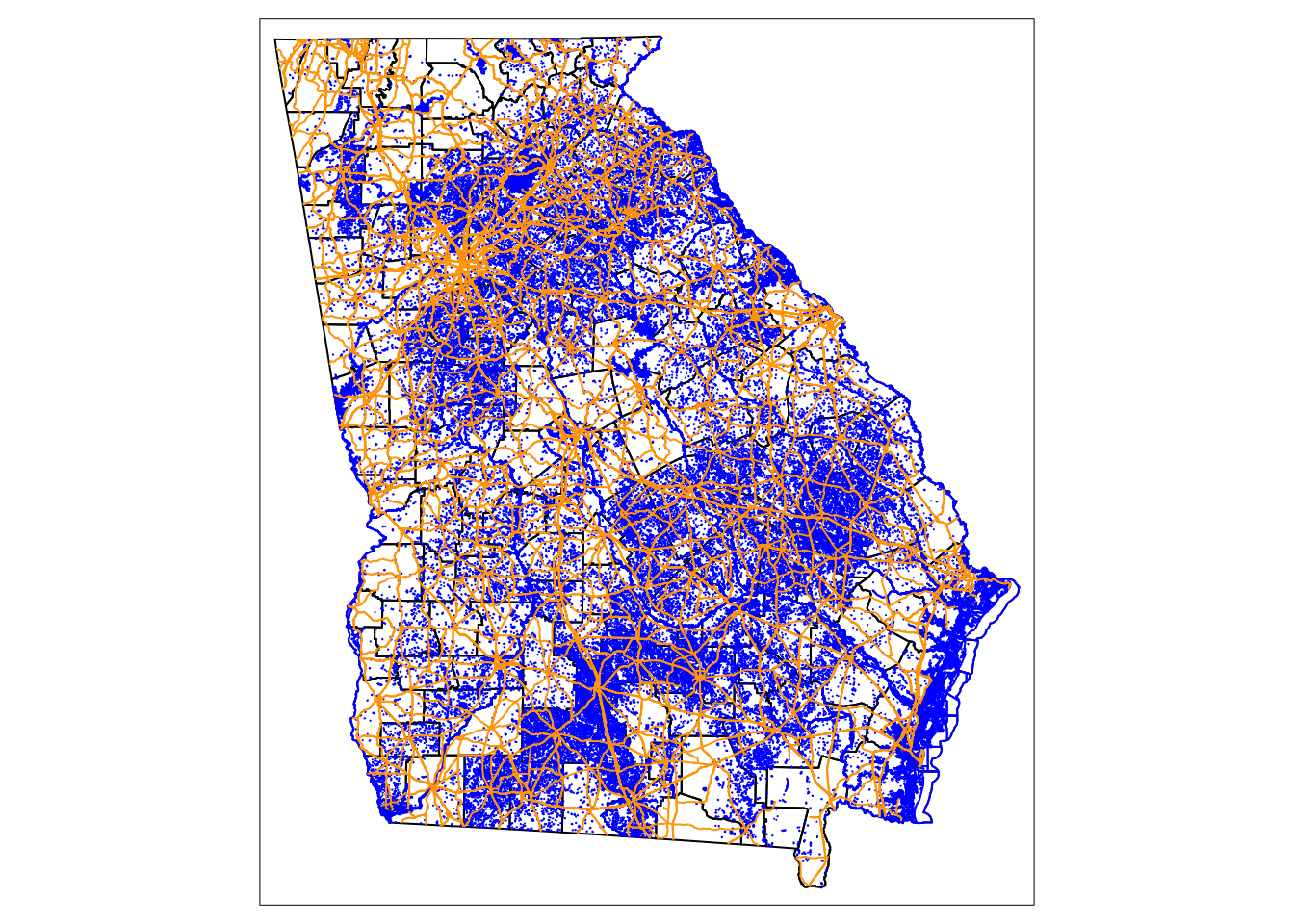

Introduction to sf

A new class of spatial objects has been defined called simple features sf. \(Sf\) objects appear as a data frame with an extra column named geometry that contains the geometrical information for the spatial part of the object. For the rest of the chapter, we will learn how to manipulate spatial features.

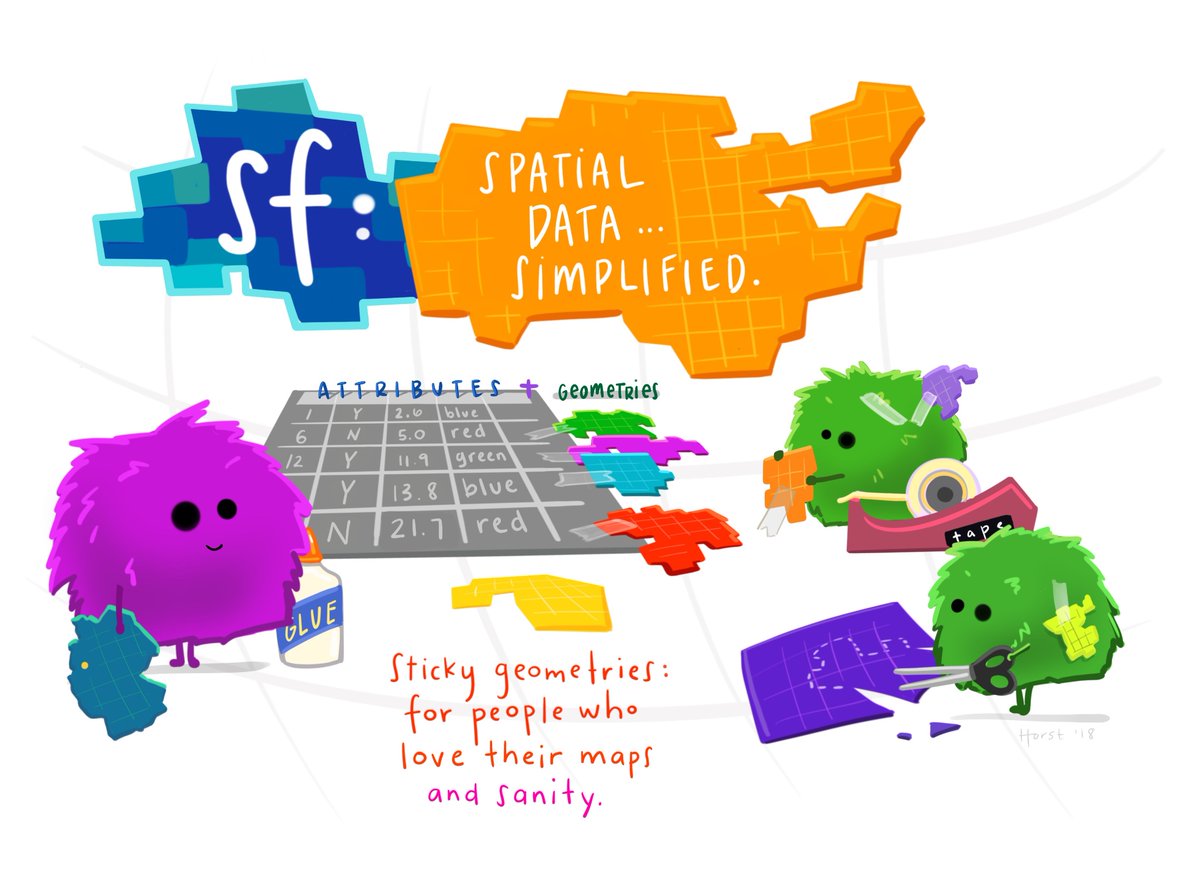
Illustration by Allison Horst, see Simple Features Blog

What is a feature?

A feature is thought of as a thing, or an object in the real world, such as a building or a tree. Features have geometry describing where on Earth the feature is located, and they have attributes, which describe other properties.

Simple feature geometry types

The following seven simple feature types are most common.

Type	Description
POINT	zero-dimensional geometry containing single point
LINESTRING	sequence of points connected by straight, non-self intersecting line pieces; one-dimensional geometry
POLYGON	geometry with a positive area (two-dimensional); sequence of points form a closed, non-self intersecting ring; the first ring denotes the exterior ring, zero or more subsequent rings denote holes in this exterior ring
MULTIPOINT	set of points; a MULTIPOINT is simple if no two Points in the MULTIPOINT are equal
MULTILINESTRING	set of linestrings
MULTIPOLYGON	set of polygons

We are going to use data from New Haven CT to work with different kinds of spatial data.

First we need to run the commands below to use the \(sf\) and \(GISTools\) packages and the New Haven data.

The New Haven data contains several \(sf\) data frames:

blocks is a data frame with population demographics broken down by block.

These attributes are saved within spatial polygons (boundaries of the blocks).
breach is a data frame with location data for public disturbances (crimes).

These attributes are saved with spatial points (x,y coordinates of the breaches).
roads contains spatial lines that mark road trajectories.

#Install and Call in the sf and GISTools libraries.

library(sf)

#Call in the newhaven data, notice this calls in multiple dataframes, examine a by clickin on them in the evironment pane

list2env(readRDS('data/newhaven.rds'), envir=environment())

<environment: R_GlobalEnv>

Below shows the blocks sf data frame which gives an example of how a \(sf\) data frame contains both spatial locations/features and the attributes of those features.

Below the geometry type is listed as a polygon which captures the boundaries of the census blocks.

It also shows the bounding box of the minimum and maximum (x,y) coordinates.

Each column denotes the spatial attributes or characteristics for each block (row), e.g., The POP1990 column reports the total population in 1990 for block 1 (pop=3071).

The last column geometry holds the spatial features of each block meaning the geographic boundaries of the polygon.

Many of the dplyr functions described above can be used on an sf data frame.

For example, we can use the \(filter()\) function to only include larger populations with POP1990> 1000.

Additionally, we can create a new variable called RentOcc that calculates the number of housing units that are renter occupied from to current variables: (a) the of housing units in \(HES\_UNITS\), and (b) the percent of renter occupied units \(P\_RENTROCC\).

#Use the filter function to subset to blocks with population >1000

# Use mutate function to create RentOcc = number of renter occ housing units.

blocks_subset <- blocks%>%
  filter(POP1990>1000) %>%
  mutate(RentOcc = HSE_UNITS * P_RENTROCC/100)

Spatial Joins combine multiple spatial data sets in the case where both data sets are spatial features.

To join a \(sf\) data set, use the \(st\_join(x,y)\) function.

The data in data set \(y\) are merged in with the data in \(x\).

If \(y\) contains values outside of \(x\) boundaries, these are discarded.

For example, if there is a location in \(y\) outside of boundaries in \(x\) it will be removed.

In the below code, we merge together the data from the block data set (population attributes of the census blocks) and the breach data set (locations of crimes).

The new data set called block_breach is a polygon object, with attributes of the polygon containing each particular point being joined as columns.

Note: If you want to join a spatial data set with a non-sf object, you can use the \(left\_join()\), \(right\_join()\) or \(full\_join()\) functions.

The \(left\_join(x,y)\) function joins all observations in \(y\) that match observations in \(x\).

The \(right\_join(x,y)\) functions joins all observations in \(x\) that match observations in \(y\).

The observations that are unmatched are discarded.

temp <- breach %>%
  st_join(blocks)

An Introduction to TMAP

This section will concentrate on learning the functions in the tmap (Tennekes, 2015).

This package focuses on mapping the spatial distribution of data attributes.

It has a similar grammar to plotting with the *ggplot package in that it seeks to handle each element of the map separately in a series of layers.

The process of making maps using tmap is one in which a series of layers are added to the map.

First \(tm_shape()\) is specified, followed by an aesthetic function that specifies what is to be plotted.

The input to \(tm_shape()\) is an sf object.

Layer 1

For example, we may want to plot the New Haven crime data.

The first layer of the plot is the geographic polygons (census block boundaries) of New Haven.

We input the \(blocks\) object in the \(tm\_shape()\) function.

We plot the borders spatial layer of the data which outlines census block boundaries.

To add custom styles to the background, type \(?tm\_style\) and \(?tm\_layout\) in the console pane to see possible options in the documentation.

?tm_style

?tm_layout

tm_shape(blocks)+

  tm_borders(col = "red", lty = "dashed") +

  tm_style("natural", bg.color = "lightblue") +
  tm_layout(title = "New Haven CT",
            title.size = 1,
            title.position = c(0.55, "top"))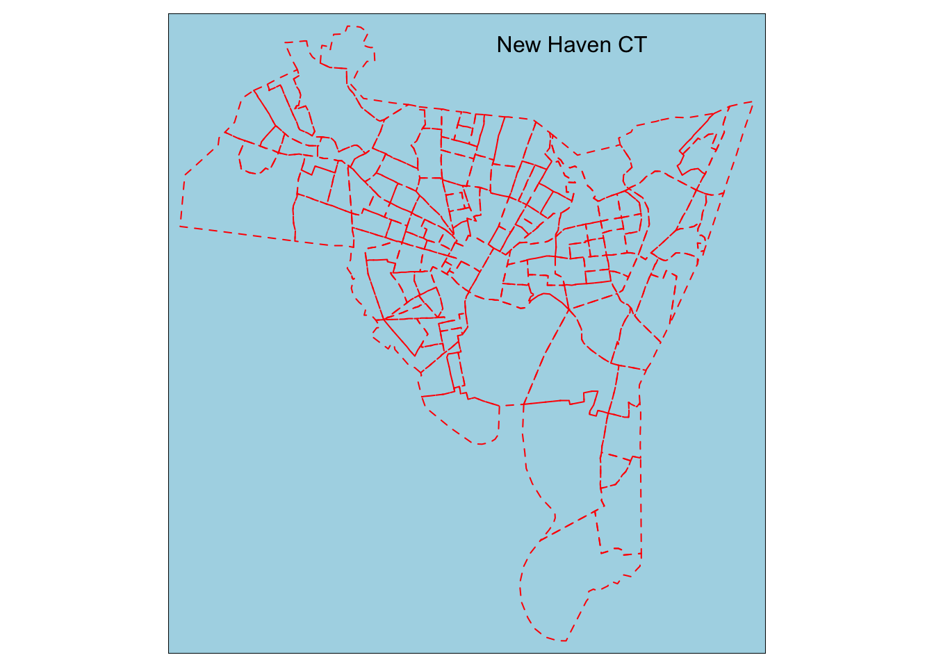

So what you can see in the above code is one set of layers for the borders where we customize the look, color, and outline.

Layer 2

A plot of geographic boundaries alone does not give much information.

We add a second layer where we can include the spatial attributes of the areas (polygons).

To add the second layer to the current plot, add another \(tm\_shape()\) function, and add the second \(sf\) object input that contains the spatial area data.

For example, here we will plot the percent of renter occupied housing units.

tm_shape(blocks)+
  tm_borders(col = "red", lty = "dashed") +
  tm_shape(blocks) +
  tm_polygons(col = "P_RENTROCC", palette = "Blues") +
  tm_layout(title = "New Haven CT",
            title.size = 1,
            title.position = c(0.55, "top"))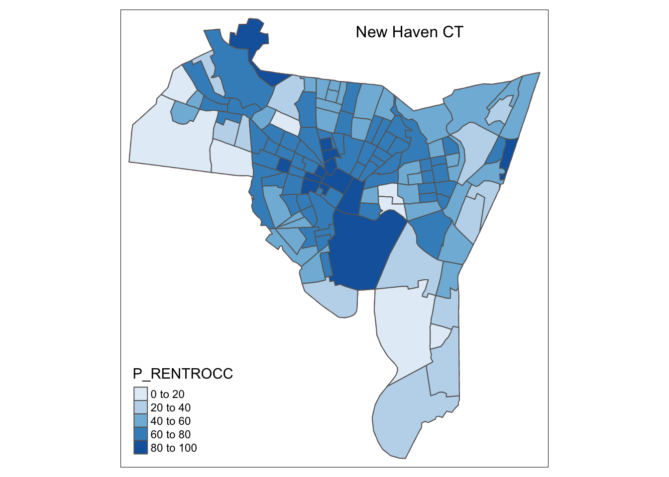

Layer 3

The third layer of the New Haven plot may include the point layer which plots the geographic coordinates of the breaches of the peace.

Extending upon layers 1 and 2, for layer 3, we use the \(breach\) data as our data layer and add point data using the \(tm\_dots()\) command.

?tm_style

?tm_layout

tm_shape(blocks)+
  tm_polygons(col = "P_RENTROCC", palette = "Blues") +
  tm_borders(col = "red", lty = "dashed") +
tm_shape(breach) +
  tm_dots(col = "blue", size = 0.1) +
  tm_layout(title = "New Haven CT",
            title.size = 1,
            title.position = c(0.55, "top"))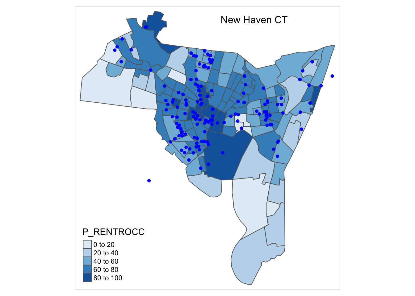

Layer 4

The fourth layer of the New Haven plot may include the lines layer which plots the roads in New Haven.

Again, add another \(tm\_shape()\) function, and add the third \(sf\) object input that contains the lines data (roads).

We add line data using the \(tm\_lines()\) command.

?tm_style

?tm_layout

st_crs(roads) <- st_crs(blocks) #this sets the projection of roads to be equal to the blocks sf dataframe

tm_shape(blocks)+
  tm_borders(col = "red", lty = "dashed") +
  tm_polygons(col = "P_RENTROCC", palette = "Blues", alpha = 0.5) +
    tm_shape(breach) +
      tm_dots(col = "blue", size = 0.1) +
        tm_shape(roads) +
          tm_lines(col = "purple", alpha = 0.5) +
  tm_layout(title = "New Haven CT",
            title.size = 1,
            title.position = c(0.55, "top"))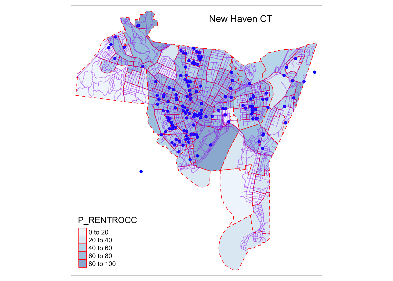

Saving Your Map

Having created a map in a window, you may now want to save the map for either printing or incorporating into a document.

There are a few simple steps to save a map in multiple formats.

If you plot the map in the Viewer pane (bottom right), you can click on the Export button to save as a pdf or copy to clipboard.
To directly save a map as a pdf/png or jep.

Above the open street map object was assigned to “om_map”.

Taking a pdf export for example, print the map after using the \(pdf()\) command, which lists the file path and the pdf file name and extension.

om_map <- tm_shape(breach)+
          tm_dots()

#Save as a pdf

pdf("mymap.pdf")

print(om_map)

off()

#Save as a jpeg

jpeg("filepath/mymap.jpg")

print(om_map)

dev.off()

Below is an example of using the \(geocode()\) function to extract US census data including coordinates and census identifiers such as census block number and FIPS code.

Note how we have changed \(method = "census"\) and we have set the \(api\_options\) to list census geographies.

Alternatively, we can use the \(reverse\_geocode()\) function to extract physical addresses from geographical pairs of latitude and longitude.

We create a data frame with \(lat\) and \(long\) values.