
Module 0: Basic R Coding
This module is a basic introduction to creating R code. This guide will outline the essential components and steps involved in performing data wrangling in RStudio. This module will not be covered during the workshop, but is a guide for those interested in coding in R.
Additional Resources
- Geocomputation with R by Robin Lovelace. This will be a recurring ‘additional resource’ as it provides lots of useful insight and strategy for working with spatial data in
R. I encourage you to browse it quickly now, but return often when you have questions about how to handle geographic data (especially of classsf) inR. - An introduction to the
ggplot2package. This is just one of dozens of great online resources introducing the grammar of graphics approach to plotting inR. - R for SAS users cheat sheet
Introduction to RStudio
- R provides a very flexible way to work with spatial and geographic data.
- To make maps in R, we need to understand characteristics and functions specific to working with spatial data:
- How to read spatial data into R.
- How to manipulate spatial data in R.
- How to visualize different kinds of spatial data, i.e., points versus areas.
- Important: We want to produce reproducible and efficient code.
This section describes the basic ways of assigning values to different types of R objects and different classes of R objects. R and RStudio must be installed on your system! Refer to Lab 0 for installation directions.
Additional Resources
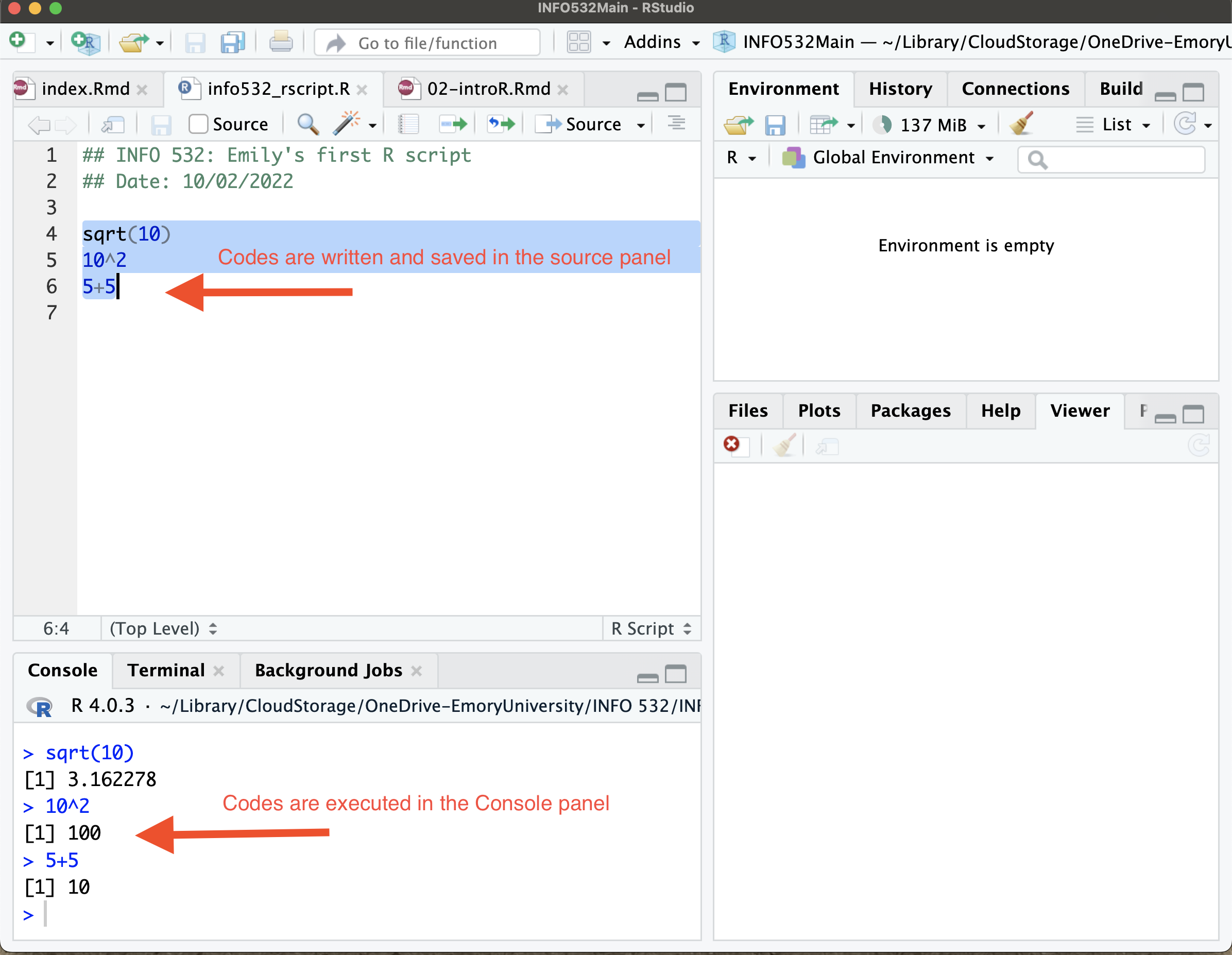
Panes in RStudio
The Source Editor can help you open, edit, execute and save these programs. It is the panel on the top left of your screen.
The console is where you can type code that is executed immediately. This is also known as the command line. It is at the bottom left of your screen.
The Environment pane is very useful as it shows you what objects (i.e. arrays, data, functions) you have in your workspace.
The last pane has a number of different tabs:
- The Files tab has a navigable file manager.
- The Packages tab shows you the packages installed.
- The Plot tab is where graphics are shown.
- The Help tab allows you to search R documentation for help.
Data Types in R
Vector data: contains multiple values within a column \(c()\).
Character data: a vector that contains text.
#We assign values to an object using <-
#We create a vector using c(). Inside the vector we insert text corresponding to city names.
cities <- c("New York City", "Atlanta", "Seattle")
cities
[1] "New York City" "Atlanta" "Seattle" - Numeric data: a vector that contains numbers.
#We create a vector using c(). Inside the vector we insert numberic values.
tree.heights <- c(4.3, 7.1, 6.3)
tree.heights
[1] 4.3 7.1 6.3- Logical data: a vector that contains TRUE or FALSE.
#We create a vector using c(). Inside the vector we insert TRUE or FALSE values.
northern <- c(TRUE, FALSE, TRUE)
northern
[1] TRUE FALSE TRUE- Factor data: a vector that contains specified categories.
#We create a vector using c(). Inside the vector we insert categorical values.
blood.pressure <- factor(c("High", "Medium", "Low", "Medium", "High", "High"),
                         levels = c("Low", "Medium", "High"))
blood.pressure
[1] High Medium Low Medium High High
Levels: Low Medium High- Matrix: numeric values contained in columns and rows, i.e., rows and columns are numeric vectors:
my_matrix <- matrix(1:4, ncol = 2, nrow = 2)
my_matrix
[,1] [,2]
[1,] 1 3
[2,] 2 4- Lists: Lists have slots for collections of different elements, which do NOT have to be the same data type
my_list <- list(cities, tree.heights, northern)
my_list[[1]]
[1] "New York City" "Atlanta" "Seattle" my_list[[2]][1] 4.3 7.1 6.3- Data Frames: A matrix contains columns and rows of numeric values. A data frame contains columns that can be different data types, i.e., real world features. The columns MUST have the same length.
df <- data.frame(char = cities, numeric = tree.heights)
df
char numeric
1 New York City 4.3
2 Atlanta 7.1
3 Seattle 6.3Functions
What is a function?
A function in R is an object that takes in a data input and performs a pre-defined operation to then output the desired result. Functions in R can be built-in or created by the user (user-defined).
- R programming language is a lot like magic…except instead of spells you have functions.
- You can think of functions as “wrappers” that condense longer code into simpler codes so you can write one line instead of 10 lines.
- You can use already written functions or create your own.
- In this book, we will use many of the pre-defined functions, but will show an example below of how to create a function.
We show examples of pre-defined functions below, which we apply to the numeric vector \(x\).
- The sqrt() function calculates the square root of the input.
- The min() function calculates the minimum value of the input.
- The max() function calculates the max value of the input.
- The summary() function calculates the statistical summaries (mean, sd, min, max, and quartiles) of the input.
x <- c(2.1, 5.4, 6.7, 1.3, 5.2)
sqrt(x)
[1] 1.449138 2.323790 2.588436 1.140175 2.280351min(x)[1] 1.3max(x)[1] 6.7summary(x) Min. 1st Qu. Median Mean 3rd Qu. Max.
1.30 2.10 5.20 4.14 5.40 6.70 To write a user-defined (custom) function, you create an R function using the function() command, and define the calculation to perform, and the output to be displayed. For example, below a function is created and assigned (<-) the name my_function. To create the function itself, the function() command is used, and the data inputs are defined as \(x\) and \(y\) (we have not defined what \(x\) and \(y\) are yet). Within the function the sum \(x\) and \(y\) is calculated and returned as an output.
my_function <- function(x,y){ #create a function called my_function

  sum <- x+y #the function calculates sum of x and y

  return(sum) #the function returns the sum
}- my_function has not been applied to any data yet. So below, we illustrate the use of my_function on both numbers and numeric vectors.
- IMPORTANTLY, do not forget to include the comma when there are multiple data inputs within the function ().
#Perform my_function on two numbers x and y.
my_function(x = 1, y = 5)
[1] 6my_function(x = 1000, y = 300)[1] 1300#Perform my_function on two numeric vectors x and y.
my_function(x = c(1,2,4,5,6), y = c(0,7,5,6,7))[1] 1 9 9 11 13my_function(x = 6, y = c(0,7,5,6,7))[1] 6 13 11 12 13Packages
What is a package? A package is simply a collections of functions.Packages also contain published data sets.
There are 16K packages in R.
One great thing about R, is that people/coders like to share what they create. They do this through packages, where you can access their pre-defined functions that have been tested, and come with help documentation.
R packages are stored and shared via the CRAN repository. The number of packages is continually growing.
To use a package, users need to install it only once, and then can continually call the package when needed. For example to install a package, use the syntax given below. It calls the package by its name, and requires all other needed packages to also be called installed \(depedencies = TRUE\).
install.packages("package_name", dependencies = TRUE, repos = "http://cran.us.r-project.org")For example, popular packages to be installed are tidyverse and dplyr.
install.packages(c("dplyr", "tidyverse"), dependencies = T)Once the packages are installed, they are saved in the local R libraries. This means they do not need to be installed again. In order to use the functions within the package, a package needs to be called using the library() function.
- For example, running the code below calls the dplyr package. There will be R statements below indicating the package has been called.
library(dplyr)To review any given function from a package, the help() or ? function will publish the documentation for the function to show required inputs, calculations, and outputs.
For example, to review the min() function, use the syntax below in the console.
help(min)Help on topic 'min' was found in the following packages:
Package Library
base /Library/Frameworks/R.framework/Resources/library
terra /Users/emilypeterson/Library/R/4.0/library
Using the first match ...?minHelp on topic 'min' was found in the following packages:
Package Library
base /Library/Frameworks/R.framework/Resources/library
terra /Users/emilypeterson/Library/R/4.0/library
Using the first match ...The bottom-right pane publishes viewer output including: help documentation, and plots. If you type the above code in the console, the viewer pane will publish the help documentation for the min function.
Introduction to DPLYR
The dplyr package is part of the tidyverse (a collection of R packages) and provides a suite of tools for manipulating and summarizing data tables and spatial data. It contains a number of functions for data transformations. DPLYR tools can be in a piping syntax that allows for a sequence of functions to happen at the same time. Think of dplyr functions as transformation spells that transform data from one thing to another.
The dplyr functions take a data frame as the first argument and layers functions using what we refer to as piping operator \(%>%\). It condenses many lines of code into a single chunk. To illustrate dplyr tools, we use the flights data set that is available from dplyr.
First, we call the tidyverse and dplyr packages
# Call libraries
library(tidyverse)
library(tmap)


# To explore more of dplyr documentation and examples use code below.
#vignette("dplyr", package = "dplyr")
Next we read in the Air Passengers data using the \(data()\) call function. This data records monthly totals of the number of international airline passengers from 1949-1960. Using the class() function, you can see what type of R object. This R object is a time-series (ts) and needs to be converted to a data frame.
#Read in the starwars data
data("AirPassengers")
#Determine the type of R object
class(AirPassengers)
[1] "ts"We transform the time series into a data frame with the below commands. The rows are the different years and the columns are months Jan-Dec.
#Transform the time series data into a data frame
air_passengers_df <- matrix(AirPassengers, ncol = 12, nrow = 12, byrow = T)
rownames(air_passengers_df) <- 1949:1960
colnames(air_passengers_df) <- c("Jan", "Feb", "Mar", "Apr", "May",
                                 "Jun", "Jul", "Aug", "Sep", "Oct",
                                 "Nov", "Dev")

air_passengers_df <- data.frame(air_passengers_df) #convert the matrix to a dataframe object
head(air_passengers_df)
Jan Feb Mar Apr May Jun Jul Aug Sep Oct Nov Dev
1949 112 118 132 129 121 135 148 148 136 119 104 118
1950 115 126 141 135 125 149 170 170 158 133 114 140
1951 145 150 178 163 172 178 199 199 184 162 146 166
1952 171 180 193 181 183 218 230 242 209 191 172 194
1953 196 196 236 235 229 243 264 272 237 211 180 201
1954 204 188 235 227 234 264 302 293 259 229 203 229What is piping? A piping syntax allows us to manipulate/mutate the data using a sequence of transformations, i.e., operations are chained together. The pipeline operator is denoted using %>%.
For example, in many cases we need to switch from wide data to long data or vice-versa. In this case, we want a monthly count as a unique row, so we want to transform this data from wide (going across columns) to long (going down rows).
Sequence of operations:
- Create a year variable in the data because we want each row to be a unique month-year combination. The \(rownames()\) function extracts the names of each row (i.e., the year corresponding to the row). The \(as.numeric()\) function turns characters into numbers.
air_passengers_df <- air_passengers_df %>%
                     mutate(year = as.numeric(rownames(air_passengers_df))) #creates a new
Create a new data set called air_passengers_long and assign it <- to the old data set.
Use the pivot_longer function from the tidyr package to convert the data to long.
air_passengers_long <- air_passengers_df %>%
  pivot_longer(cols = 1:12, names_to =  "Month", values_to = "count")

head(air_passengers_long)
# A tibble: 6 × 3
year Month count
<dbl> <chr> <dbl>
1 1949 Jan 112
2 1949 Feb 118
3 1949 Mar 132
4 1949 Apr 129
5 1949 May 121
6 1949 Jun 135If we want to filter the data to only include the month of January, we use the \(filter()\) function shown below in the first line of code. If we want to filter to Jan and the year must be greater than 1955, we can use the second line of code.
#Use the filter function to subset only to data for Jan.
jan_only_df <- air_passengers_long %>%
  filter(Month == "Jan")

#Use the filter function to subset only to data for Jan AND for years > 1955
jan1955_only_df <- air_passengers_long %>%
  filter(Month == "Jan" & year > 1955)
We can arrange the dataset in order of a variable (e.g., by year) using the arrange() function. \(arrange()\) orders the rows by the values selected in the columns. It sorts from smallest to largest.
#Arrange the data by year
arrange_df <- air_passengers_long %>%
  arrange(desc(year))
head(arrange_df)
# A tibble: 6 × 3
year Month count
<dbl> <chr> <dbl>
1 1960 Jan 417
2 1960 Feb 391
3 1960 Mar 419
4 1960 Apr 461
5 1960 May 472
6 1960 Jun 535Two important functions are the mutate() and summarize() functions. We create new variables (not already defined) using the \(mutate()\) function. For example, if we want to create a new logical variable that is TRUE if year > 1955, and FALSE otherwise, we can use the code below, which uses the combination of the \(mutate()\) and \(ifelse()\) functions.
#Create a new logical variable using the mutate function, if year > 1955 then TRUE else FALSE.
mutate_df <- air_passengers_df %>%
  mutate(year_indicator = ifelse(year > 1955, TRUE, FALSE))
If we want to summarize the data, we can use the summarize() function. For example, if we want the mean number of passengers by year, we first use the group_by() function to define which groups we want to summarize, in this case it is year. Then we use the summarize() function to define what summaries we want, e.g., mean, sd, median, and others.
# First group_by year to group the data by year variable.
#Then summarize the mean number of passengers to get the mean BY year.
summary_df <- air_passengers_long %>%
  group_by(year) %>%
  summarize(mean_number = mean(count))

head(summary_df)
# A tibble: 6 × 2
year mean_number
<dbl> <dbl>
1 1949 127.
2 1950 140.
3 1951 170.
4 1952 197
5 1953 225
6 1954 239.The piping syntax allows us to perform commands in sequence in one code chunk versus multiple transformations. The code below shows how we can combine comands into one executable function. Note: The sequence of commands is important. For example, we first must create the year variable using the \(mutate()\) function before we filter by year.
For example, the chunk below shows all the steps above as one sequential workflow. No need to break things into multiple datasets.
air_passengers_df <- matrix(AirPassengers, ncol = 12, nrow = 12, byrow = T)
rownames(air_passengers_df) <- 1949:1960
colnames(air_passengers_df) <- c("Jan", "Feb", "Mar", "Apr", "May",
                                 "Jun", "Jul", "Aug", "Sep", "Oct",
                                 "Nov", "Dev")

air_passengers_mean_data <- data.frame(matrix(AirPassengers, ncol = 12, nrow = 12, byrow = T)) %>%
  rename(c("Jan" = "X1", "Feb" = "X2", "Mar" = "X3", "Apr" = "X4", "May" = "X5",
                                 "Jun" = "X6", "Jul" = "X7", "Aug" = "X8",
                                  "Sep" = "X9", "Oct" = "X10",
                                 "Nov" = "X11", "Dec" = "X12")) %>%
  mutate(year= c(1949:1960),
         year_indicator = ifelse(year > 1955, TRUE, FALSE)) %>%
  pivot_longer(cols = 1:12, names_to =  "Month", values_to = "count") %>%
  arrange(year) %>%
  group_by(year) %>%
  summarize(mean_number = mean(count))

air_passengers_mean_data
# A tibble: 12 × 2
year mean_number
<int> <dbl>
1 1949 127.
2 1950 140.
3 1951 170.
4 1952 197
5 1953 225
6 1954 239.
7 1955 284
8 1956 328.
9 1957 368.
10 1958 381
11 1959 428.
12 1960 476.