5 Vector Spaces
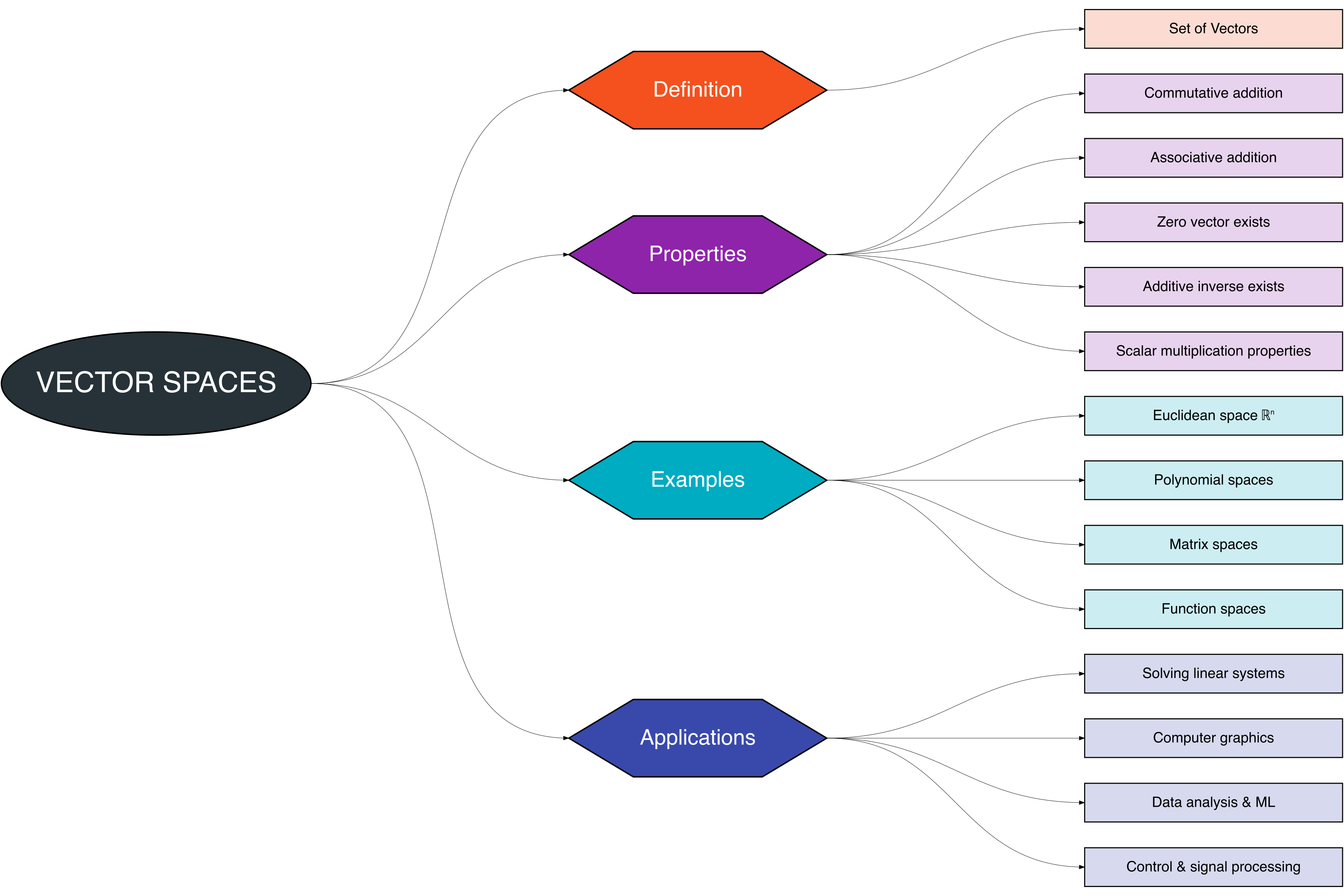
In this chapter, we explore the concept of vector spaces and their fundamental properties. A Figure 5.1 provides a structured overview of the key topics discussed:
Vector spaces are a fundamental concept in linear algebra and have significant applications in mining engineering. A vector space is a set of vectors that is closed under vector addition and scalar multiplication, satisfying properties such as commutativity, associativity, the existence of a zero vector, and additive inverses.
In the context of mining:
- Ore Modeling: Vectors can represent ore grades at different locations in a mine. This allows for geostatistical analysis and estimation of ore quality across a deposit.
- Resource Allocation: Equipment, labor, and material assignments can be expressed as vectors, enabling efficient planning and optimization of mining operations.
- Geospatial Analysis: Positions of mining points, boreholes, or sensors are naturally represented in \(\mathbb{R}^3\), allowing for 3D modeling, visualization, and spatial transformations.
- Production Planning: Production rates over time can be modeled as vectors, facilitating adjustments and optimization of extraction schedules.
- Risk Assessment: Safety levels or hazard indices across mine zones can be represented as vectors. Norms of these vectors help quantify overall risk and guide mitigation strategies.
Vector spaces provide a rigorous mathematical framework that underpins linear system solutions, optimization, and modeling in mining. They also enable a unified understanding of matrices, polynomials, and function spaces, making them essential for advanced mining analytics and operational decision-making [1], [2].
5.1 Definition
A set \(V\) is a vector space over a field \(\mathbb{F}\) if it satisfies the following conditions:
Closure under addition:
For all \(u, v \in V\), \(u + v \in V\).Closure under scalar multiplication:
For all \(v \in V\) and \(c \in \mathbb{F}\), \(c v \in V\).Zero vector exists:
There exists a vector \(0 \in V\) such that \(v + 0 = v\) for all \(v \in V\).Additive inverse exists:
For each \(v \in V\), there exists \(-v \in V\) such that \(v + (-v) = 0\).Commutativity of addition:
\(u + v = v + u\) for all \(u, v \in V\).Associativity of addition:
\((u + v) + w = u + (v + w)\) for all \(u, v, w \in V\).Distributivity of scalar multiplication over vector addition:
\(a(u+v) = au + av\).Distributivity of scalar multiplication over field addition:
\((a+b)v = av + bv\).Compatibility of scalar multiplication:
\((ab)v = a(bv)\).Identity element of scalar multiplication:
\(1v = v\).
These properties ensure that vector addition and scalar multiplication behave in a consistent and predictable way.
5.2 Properties
Vector spaces exhibit several important properties that can be used to simplify analysis and computations:
| Property | Description |
|---|---|
| Commutative Addition | \(u + v = v + u\) |
| Associative Addition | \((u + v) + w = u + (v + w)\) |
| Zero Vector | Exists \(0 \in V\) such that \(v + 0 = v\) |
| Additive Inverse | For \(v \in V\), \(-v \in V\) satisfies \(v + (-v) = 0\) |
| Scalar Multiplication | \(c v \in V\) for \(c \in \mathbb{F}\) and \(v \in V\) |
| Distributive Laws | \(a(u+v) = au + av\), \((a+b)v = av + bv\) |
| Compatibility | \((ab)v = a(bv)\) |
| Multiplicative Identity | \(1v = v\) |
5.3 Examples of Vector Spaces
Vector spaces can take many forms. Common examples include:
Euclidean space \(\mathbb{R}^n\)
The set of all \(n\)-dimensional real vectors:
\[ \mathbb{R}^n = \{ x = [x_1, x_2, ..., x_n]^T : x_i \in \mathbb{R} \} \]Polynomial spaces
All polynomials of degree \(\le n\):
\[ P_n = \{ p(x) = a_0 + a_1 x + ... + a_n x^n : a_i \in \mathbb{R} \} \]Matrix spaces
All \(m \times n\) matrices over \(\mathbb{R}\):
\[ M_{m \times n} = \{ A = [a_{ij}] : a_{ij} \in \mathbb{R} \} \]Function spaces
Continuous functions on an interval \([a, b]\):
\[ C[a,b] = \{ f : [a,b] \to \mathbb{R}, f \text{ continuous} \} \]
5.4 Applications
Vector spaces provide a powerful framework to model and analyze mining operations. Examples include:
5.4.1 Ore Grade Estimation
Ore grades at different locations in a mine can be represented as vectors:
\[
\mathbf{g} = [g_1, g_2, g_3, ..., g_n]^T
\]
where \(g_i\) is the ore grade at location \(i\).
Using vector operations and interpolation techniques (e.g., Kriging), we can estimate ore quality across the deposit.
5.4.2 Resource Allocation
Equipment, labor, and material allocation can be modeled as vectors:
\[
\mathbf{x} = [x_1, x_2, ..., x_m]^T
\]
where \(x_i\) represents the amount of resource \(i\) assigned.
Vector addition and scalar multiplication help in scaling and combining allocation strategies for optimal production.
5.4.3 Geospatial Modeling
Positions of mining points, boreholes, or sensors can be expressed in \(\mathbb{R}^3\):
\[
\mathbf{p}_i = [x_i, y_i, z_i]^T
\]
where \((x_i, y_i, z_i)\) are coordinates of point \(i\).
Operations in vector spaces enable transformations, rotations, and translations for 3D mine modeling and visualization.
5.4.4 Production Planning
Production rates over multiple time periods can be represented as vectors:
\[
\mathbf{r} = [r_1, r_2, ..., r_T]^T
\]
Vector addition allows combining different schedules, while scalar multiplication adjusts production levels to meet targets efficiently.
5.4.5 Safety and Risk Analysis
Risk levels of different zones in a mine can be modeled as vectors:
\[
\mathbf{s} = [s_1, s_2, ..., s_k]^T
\]
Vector norms (\(\|\mathbf{s}\|\)) provide a measure of overall risk, and vector operations help in evaluating mitigation strategies across zones.
Summary:
Using vector spaces, mining engineers can represent complex multi-dimensional data, perform calculations efficiently, and optimize operational decisions. This provides a strong mathematical foundation for geostatistics, production planning, and risk assessment in mining.
References
[1]
Meyer, C. D., Matrix analysis and applied linear algebra, SIAM, 2000
[2]
Golub, G. H. and Loan, C. F. V., Matrix computations, Johns Hopkins University Press, Baltimore, MD, 2013