1  Systems of Linear Equations

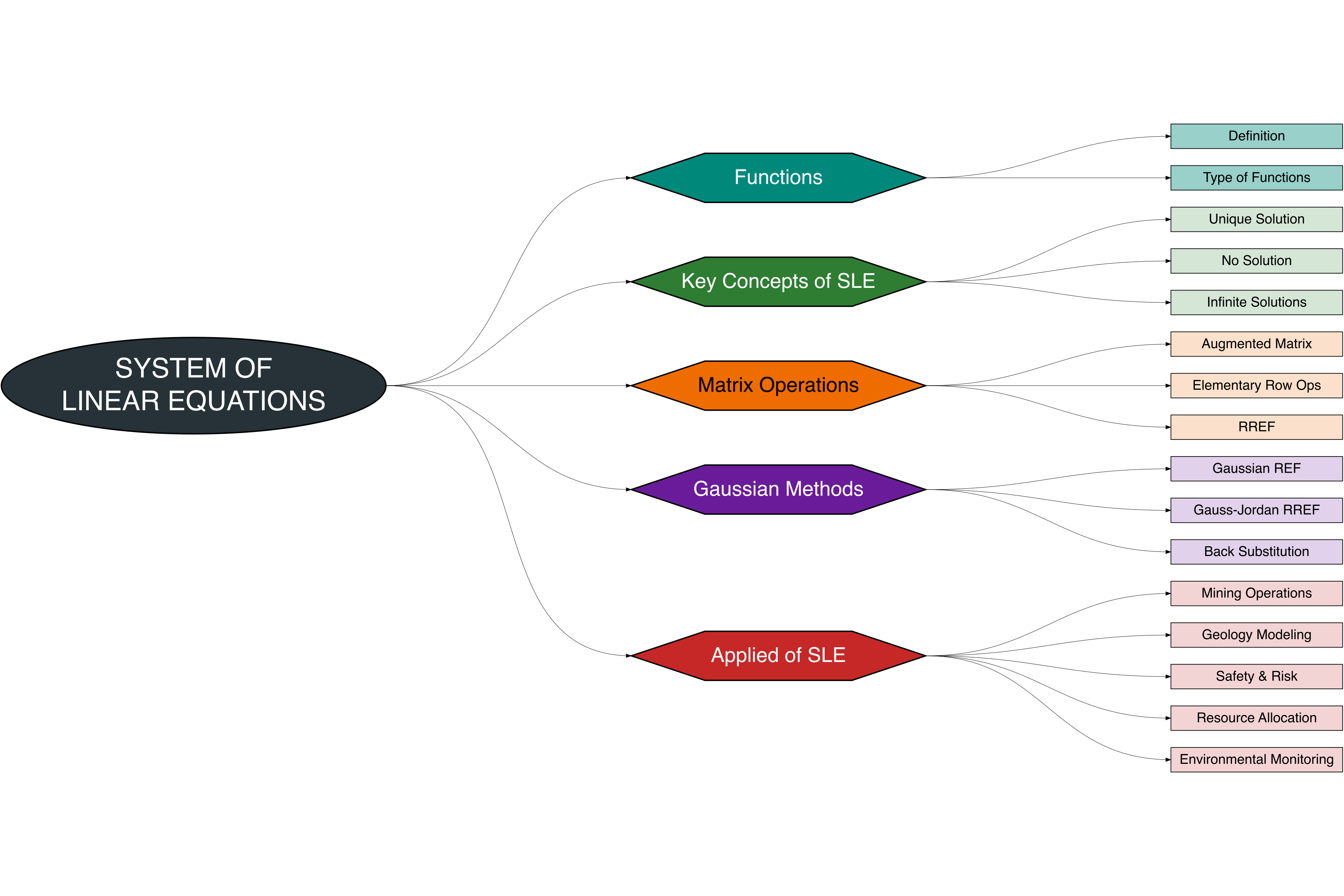
Linear algebra begins with one of its most fundamental topics: Systems of Linear Equations (SLE). These systems appear everywhere in mining engineering, geosciences, mineral processing, and numerical modeling [1]–[4]. Figure 1.1 shows a mind map of SLE and its main concepts, operations, and applications in mining engineering.

Figure 1.1: Mind Map of System of Linear Equations

1.1 Functions to Linear Equations

A function is a relation that connects each input value to exactly one output value [5], [6]. In mathematics, a function is often written as:

\[ f(ax)=b \]

• \(a:\) Coefficient of the independent variable
  
• \(x:\) Input (independent variable)
  
• \(b:\) Output (dependent variable)

Functions are the foundation of linear equations, since every linear equation can be seen as a special type of function [2].

Note:

A linear equation is a function where the variables only appear to the first power and are not multiplied together [1]. In general form:

\[ a_1x_1 + a_2x_2 + \dots + a_nx_n = b \]

where \(a_1, a_2, \dots, a_n\) are constants (coefficients), and \(b\) is a constant term.

• With 1 variable: \(a_1x_1 = b\)
  
• With 2 variables: \(a_1x_1 + a_2x_2 = b\)
  
• With N variables: \(a_1x_1 + a_2x_2 + \dots + a_nx_n = b\)

1.2 System of Linear Equations

A SLE is a collection of two or more linear equations involving the same set of variables. The goal is to find values of the variables that satisfy all equations at once [1], [2].

General form:

\[ \begin{aligned} a_{11}x_1 + a_{12}x_2 + \dots + a_{1n}x_n &= b_1 \\ a_{21}x_1 + a_{22}x_2 + \dots + a_{2n}x_n &= b_2 \\ \vdots \quad & \quad \vdots \\ a_{m1}x_1 + a_{m2}x_2 + \dots + a_{mn}x_n &= b_m \end{aligned} \]

• \(m =\) number of equations
  
• \(n =\) number of variables

1.3 Key Concepts of SLE

1.3.1 Unique Solution

The system has exactly one solution. This occurs when the equations represent lines (or planes in higher dimensions) that intersect at a single point [1], [2].

Example

Consider the following system:

\[ \begin{aligned} x_1 + x_2 &= 5 \\ 2x_1 - x_2 &= 1 \end{aligned} \]

Solution

Solving the System:

\[ \begin{aligned} x_1 + x_2 &= 5 & \text{(first equation)} \\[5pt] x_2 &= 5 - x_1 & \text{(express $x_2$ in terms of $x_1$)} \\[5pt] 2x_1 - x_2 &= 1 & \text{(second equation)} \\[10pt] 2x_1 - (5 - x_1) &= 1 & \text{(substitute $x_2 = 5 - x_1$)} \\[5pt] 2x_1 - 5 + x_1 &= 1 & \text{(simplify)} \\[5pt] 3x_1 - 5 &= 1 & \text{(combine like terms)} \\[5pt] 3x_1 &= 6 & \text{(move constant to RHS)} \\[5pt] x_1 &= 2 & \text{(solve for $x_1$)} \\[10pt] x_2 &= 5 - 2 = 3 & \text{(substitute $x_1=2$ into $x_2=5-x_1$)} \\[5pt] (x_1, x_2) &= (2,3) & \text{(final solution: intersection point)} \end{aligned} \]

Conclusion:
The unique solution is:
\[ (x_1, x_2) = (2,3) \]

Solution: Visualization

We can visualize both equations as straight lines in the coordinate plane. The intersection point of these lines represents the unique solution [7].

Figure 1.2: Interactive visualization of the system: x1 + x2 = 5 and 2x1 − x2 = 1

1.3.2 No Solution

The system has no solution. This happens when the equations are inconsistent, typically represented by parallel lines that never intersect [1].

Example

Consider the following system:

\[ \begin{aligned} x_1 + x_2 &= 4 \\ x_1 + x_2 &= 6 \end{aligned} \]

Question:
Is there a pair \((x_1, x_2)\) that satisfies both equations simultaneously?

Solution

Let’s try solving:

\[ \begin{aligned} x_1 + x_2 &= 4 \\ x_1 + x_2 &= 6 \end{aligned} \]

Subtracting (1) from (2):

\[ (x_1 + x_2) - (x_1 + x_2) = 6 - 4 \]

\[ 0 = 2 \quad \text{(contradiction)} \]

Since we arrive at a contradiction, the system is inconsistent and has no solution.

Solution: Visualization

Graphically, the two equations are parallel lines. Since they never intersect, there is no common solution point.

Figure 1.3: Interactive visualization of the inconsistent SLE: x1 + x2 = 4 and x1 + x2 = 6

1.3.3 Infinite Solutions

The system has infinitely many solutions. This occurs when the equations are dependent, meaning they represent the same line (or plane) written in different forms [1].

Example

Consider the following system:

\[ \begin{aligned} x_1 + x_2 &= 5 \\ 2x_1 + 2x_2 &= 10 \end{aligned} \]

Question:
How many solutions does this system have?

Solution

Let’s check:

\[ \begin{aligned} x_1 + x_2 &= 5 \\ 2x_1 + 2x_2 &= 10 \end{aligned} \]

Notice that equation (2) is just twice equation (1):

\[ 2(x_1 + x_2) = 2 \times 5 = 10 \]

Thus, both equations describe the same line.
This means there are infinitely many solutions.

Every pair \((x_1, x_2)\) such that

\[ x_1 + x_2 = 5 \]

is a valid solution. For example:

• \((x_1, x_2) = (0,5)\)
  
• \((x_1, x_2) = (2,3)\)
  
• \((x_1, x_2) = (4,1)\)
  
• etc.
  

Solution: Visualization

Graphically, both equations represent the same line. Hence, instead of intersecting at a single point, they overlap completely, which means infinitely many solutions.

Figure 1.4: Interactive visualization of the dependent SLE: x1 + x2 = 5 and 2x1 + 2x2 = 10

1.4 Matrix Operations

In the final part of Matrix Operations, we focus on three main concepts that are widely used to solve systems of linear equations (SLE): Augmented Matrix, Elementary Row Operations (ERO), and Reduced Row Echelon Form (RREF). These topics provide both the theoretical foundation and practical algorithms used in engineering and numerical computation [1], [3], [6].

1.4.1 Augmented Matrix

Definition: An augmented matrix is a compact representation of a linear system where the coefficient matrix and the constant (right-hand side) vector are written side-by-side, separated by a vertical bar. This representation simplifies applying row operations and implementing algorithms like Gaussian elimination [1].

\[ \begin{cases} a_1x_1 + a_2x_2 = b_1 \\[6pt] a_3x_1 + a_4x_2 = b_2 \end{cases} \] The system can be written in augmented matrix form:

\[ \left[\begin{array}{cc|c} a_1 & a_2 & b_1 \\[6pt] a_3 & a_4 & b_2 \end{array}\right] \]

1.4.2 Elementary Row Operations

There are three elementary row operations that do not change the solution set of a linear system [6]:

1. Swap two rows: \(R_i \leftrightarrow R_j\).
   
2. Multiply a row by a nonzero scalar: \(R_i \leftarrow k R_i, \; k \neq 0\).
   
3. Add a multiple of one row to another: \(R_i \leftarrow R_i + k R_j\).

These operations are used to transform the augmented matrix toward Row Echelon Form (REF) or Reduced Row Echelon Form (RREF). Note on determinants (square coefficient matrices): swapping rows changes the sign of determinant, scaling a row scales the determinant, and adding a multiple of another row does not change the determinant [3].

Three basic row operations that do not change the solution set of an SLE:

Step 1: Eliminate entry (2,1)

\[ R_2 \to R_2 - \frac{a_3}{a_1}R_1 \]

\[ \left[\begin{array}{cc|c} a_1 & a_2 & b_1 \\[6pt] 0 & a_4 - \tfrac{a_3}{a_1}a_2 & b_2 - \tfrac{a_3}{a_1}b_1 \end{array}\right] \]

Step 2: Normalize the pivot in row 2

\[ R_2 \to \frac{1}{a_4 - \tfrac{a_3}{a_1}a_2}R_2 \]

\[ \left[\begin{array}{cc|c} a_1 & a_2 & b_1 \\[6pt] 0 & 1 & \dfrac{b_2 - \tfrac{a_3}{a_1}b_1}{a_4 - \tfrac{a_3}{a_1}a_2} \end{array}\right] \]

Step 3: Eliminate entry (1,2)

\[ R_1 \to R_1 - a_2R_2 \]

\[ \left[\begin{array}{cc|c} 1 & 0 & \dfrac{b_1a_4 - a_2b_2}{a_1a_4 - a_2a_3} \\[8pt] 0 & 1 & \dfrac{a_1b_2 - a_3b_1}{a_1a_4 - a_2a_3} \end{array}\right] \]

Note:

• EROs preserve the solution set.
  
• Determinant effects (for square matrices):
  • Swapping rows ↦ changes the sign of determinant.
    
  • Multiplying a row by \(k\) ↦ determinant multiplied by \(k\).
    
  • Adding a multiple of another row ↦ determinant unchanged.
    

1.4.3 Reduced Row Echelon Form

RREF is a simplified form of a matrix obtained by applying elementary row operations (EROs), making the solution easy to read.

Characteristics of RREF [1], [6]:

1. Each nonzero row has a leading 1 (the first nonzero entry).
   
2. Each leading 1 appears to the right of the leading 1 in the row above.
   
3. Each pivot column has zeros in all other positions.
   
4. Any zero rows (if present) are placed at the bottom.

Closed-form solution (2×2 system).

For the system \[ \begin{aligned} a_1 x_1 + a_2 x_2 &= b_1, \\ a_3 x_1 + a_4 x_2 &= b_2, \end{aligned} \]

the solution is: \[ x_1 = \frac{b_1a_4 - a_2b_2}{a_1a_4 - a_2a_3}, \quad x_2 = \frac{a_1b_2 - a_3b_1}{a_1a_4 - a_2a_3}. \]

Gaussian elimination reduces a system to row echelon form (REF), which is almost upper triangular, and then solves by back substitution. Gauss–Jordan elimination continues the process until the matrix is in RREF, allowing the solution to be read directly from the augmented matrix without back substitution.

1.4.4 Step-by-Step Example

Solve:

\[ \begin{cases} x + 2y = 5\\[4pt] 3x - y = 4 \end{cases} \]

Initial augmented matrix: \[ \left[\begin{array}{cc|c} 1 & 2 & 5\\[4pt] 3 & -1 & 4 \end{array}\right] \]

Step 1 — Eliminate (2,1): \(R_2 \leftarrow R_2 - 3R_1\)

\[ \left[\begin{array}{cc|c} 1 & 2 & 5\\[4pt] 0 & -7 & -11 \end{array}\right] \]

Step 2 — Make leading 1 in row 2: \(R_2 \leftarrow (-\tfrac{1}{7})R_2\).

\[ \left[\begin{array}{cc|c} 1 & 2 & 5\\[4pt] 0 & 1 & \tfrac{11}{7} \end{array}\right] \]

Step 3 — Eliminate above leading 1: \(R_1 \leftarrow R_1 - 2R_2\).

\[ \left[\begin{array}{cc|c} 1 & 0 & \tfrac{13}{7}\\[6pt] 0 & 1 & \tfrac{11}{7} \end{array}\right] \]

Final solution:

\[ x = \tfrac{13}{7}, \quad y = \tfrac{11}{7} \]

1.5 Gaussian REF

Gaussian methods are systematic ways to solve systems of linear equations (SLE).
The main idea: simplify the system step by step (forward elimination) until the matrix is in Row Echelon Form (REF), then solve by back-substitution [1], [3].

1.5.1 Row Echelon Form (REF)

The Row Echelon Form (REF) is an intermediate step in Gaussian elimination with the following properties [6]:

• The matrix looks like a triangle: all entries below each pivot are zero.
  
• Each pivot (the first nonzero entry in a row) appears to the right of the pivot in the row above.
  
• Any rows consisting entirely of zeros appear at the bottom of the matrix.

REF is obtained by forward elimination (elementary row operations). After REF is reached, use back-substitution starting from the bottom row to compute the solution.

Example

Consider the following augmented matrix:

\[ \left[\begin{array}{ccc|c} 1 & 2 & 1 & 4 \\[4pt] 0 & -5 & 1 & -1 \end{array}\right] \]

This matrix represents the system:

\[ \begin{aligned} x_1 + 2x_2 + x_3 &= 4 \\ -5x_2 + x_3 &= -1 \end{aligned} \]

• In the first row, the pivot is the coefficient of \(x_1\), which is \(1\).
• In the second row, the pivot is \(-5\) (for \(x_2\)), and the entry below the pivot in the first column is already \(0\).
• Therefore the matrix is already in Row Echelon Form.

Steps to obtain REF (Gaussian elimination — general procedure)

1. Choose a pivot column: Start from the leftmost column that has a nonzero entry.
   
2. Select a pivot row: Choose a row with a nonzero entry in that column (often the current row).
   
3. (Optional) Scale pivot to 1: Divide the pivot row by the pivot value if you want a leading 1 (not required for REF; required for RREF).
   
4. Eliminate below pivot: Use row operations to make every entry below the pivot equal to \(0\).
   
5. Move to the submatrix below and to the right: Repeat the process for the remaining rows and columns.
   
6. Move zero rows to the bottom: If any row becomes all zeros, place it at the bottom of the matrix.

Row operations allowed (do not change solution set):

• \(R_i \leftrightarrow R_j\) (swap two rows)
  
• \(R_i \leftarrow k R_i\) (multiply a row by a nonzero scalar \(k\))
  
• \(R_i \leftarrow R_i + k R_j\) (add a multiple of one row to another)

Solution

From the REF example we have:

\[ \begin{aligned} (1)\ & x_1 + 2x_2 + x_3 = 4 \\ (2)\ & -5x_2 + x_3 = -1 \end{aligned} \]

Solve (2) for \(x_3\) in terms of \(x_2\):

\[ -5x_2 + x_3 = -1 \quad \Longrightarrow \quad x_3 = 5x_2 - 1 \]

Substitute into (1):

\[ x_1 + 2x_2 + (5x_2 - 1) = 4 \]

Simplify:

\[ x_1 + 7x_2 - 1 = 4 \quad \Longrightarrow \quad x_1 + 7x_2 = 5 \]

Thus:

\[ x_1 = 5 - 7x_2, \qquad x_3 = 5x_2 - 1 \]

Parameterize the solution by letting \(x_2 = t\) (free parameter). Then

\[ \begin{aligned} x_1 &= 5 - 7t \\ x_2 &= t \\ x_3 &= 5t - 1 \end{aligned} \] for any real number \(t\).

1.5.2 Gauss–Jordan (RREF)

The Reduced Row Echelon Form (RREF) is the final stage of Gaussian elimination, obtained using the Gauss–Jordan method. It goes further than Row Echelon Form (REF) by ensuring that each pivot column contains a leading 1 with zeros both below and above it [1], [6].

Key Properties of RREF:

• Each pivot (leading 1) is the only nonzero entry in its column.
  
• The pivot in each successive row appears to the right of the pivot in the row above.
  
• Rows consisting entirely of zeros, if any, are always at the bottom.
  
• This is the simplest form of a system: the solution can be read directly without back-substitution.

Example

\[ \left[\begin{array}{ccc|c} 1 & 0 & 0 & b_1 \\[6pt] 0 & 1 & 0 & b_2 \\[6pt] 0 & 0 & 1 & b_3 \end{array}\right] \]

This corresponds to the system:

\[ \begin{aligned} x_1 &= b_1 \\ x_2 &= b_2 \\ x_3 &= b_3 \end{aligned} \]

So the unique solution is:

\[ x_1 = b_1, \quad x_2 = b_2, \quad x_3 = b_3 \]

Steps to Obtain RREF (Gauss–Jordan Elimination)

1. Transform to REF: Use Gaussian elimination to create a triangular form with pivots.
   

2. Scale pivots to 1: Divide each pivot row so that the pivot element becomes exactly 1.
   

3. Eliminate above pivots: Use row operations to make all entries above each pivot equal to 0.
   

4. Check consistency: If a row becomes

   \[ [0 \;\; 0 \;\; 0 \;|\; b], \quad b \neq 0, \]

   then the system is inconsistent (no solution).
   

5. Read solution: Once in RREF, the solution can be read directly.

Consider the system:

\[ \begin{aligned} x_1 + 2x_2 + x_3 &= 4 \\ -5x_2 + x_3 &= -1 \end{aligned} \]

The RREF of its augmented matrix is:

\[ \left[\begin{array}{ccc|c} 1 & 0 & 7 & 5 \\[6pt] 0 & 1 & -\tfrac{1}{5} & \tfrac{1}{5} \end{array}\right] \]

This means:

\[ \begin{aligned} x_1 + 7x_3 &= 5 \\ x_2 - \tfrac{1}{5}x_3 &= \tfrac{1}{5} \end{aligned} \]

Rewriting:

\[ \begin{aligned} x_1 &= 5 - 7x_3 \\ x_2 &= \tfrac{1}{5} + \tfrac{1}{5}x_3 \end{aligned} \]

Let \[x_3 = t\] (a free parameter). Then the solution set is:

\[ \begin{bmatrix} x_1 \\ x_2 \\ x_3 \end{bmatrix} = \begin{bmatrix} 5 \\ \tfrac{1}{5} \\ 0 \end{bmatrix} + t \begin{bmatrix} -7 \\ \tfrac{1}{5} \\ 1 \end{bmatrix}, \quad t \in \mathbb{R}. \]

1.5.3 Back Substitution

When we stop at Row Echelon Form (REF) rather than continuing to RREF, we must use back substitution to solve the system [1], [6].

• Start solving from the bottom row (which involves fewer variables).
  
• Substitute upward step by step until all variables are expressed (or expressed in terms of free parameters).

Example

Consider the augmented matrix in REF:

\[ \left[\begin{array}{ccc|c} 1 & 2 & 1 & 4 \\[6pt] 0 & -5 & 1 & -1 \end{array}\right] \]

This corresponds to the system:

\[ \begin{aligned} x_1 + 2x_2 + x_3 &= 4 \\ -5x_2 + x_3 &= -1 \end{aligned} \]

Step 1: Start with the bottom row, From equation (2):

\[ -5x_2 + x_3 = -1 \]

Rearrange to express \(x_2\) in terms of \(x_3\):

\[ x_2 = \frac{1 + x_3}{5} \]

Step 2: Substitute into the first row, Plug \(x_2 = \tfrac{1+x_3}{5}\) into equation (1):

\[ x_1 + 2\left(\frac{1+x_3}{5}\right) + x_3 = 4 \]

Simplify:

\[ x_1 + \frac{2}{5} + \frac{2}{5}x_3 + x_3 = 4 \]

\[ x_1 + \frac{7}{5}x_3 + \frac{2}{5} = 4 \]

\[ x_1 = 4 - \frac{2}{5} - \frac{7}{5}x_3 \]

\[ x_1 = \frac{18}{5} - \frac{7}{5}x_3 \]

Step 3: Express the solution set

Let \(x_3 = t \in \mathbb{R}\) (a free parameter). Then:

\[ \begin{aligned} x_1 &= \frac{18}{5} - \frac{7}{5}t \\ x_2 &= \frac{1+t}{5} \\ x_3 &= t \end{aligned} \]

Final Solution (Parametric Form)

\[ \begin{bmatrix} x_1 \\ x_2 \\ x_3 \end{bmatrix} = \begin{bmatrix} \tfrac{18}{5} \\ \tfrac{1}{5} \\ 0 \end{bmatrix} + t \begin{bmatrix} -\tfrac{7}{5} \\ \tfrac{1}{5} \\ 1 \end{bmatrix}, \quad t \in \mathbb{R}. \]

1.6 Applied of SLE

Systems of Linear Equations (SLE) are widely used in real-world mining and geoscience problems.
They provide a mathematical way to represent constraints and balances in production, blending, transport, and geological modeling.

1.6.1 Mining Operations

In mining operations, linear equations often appear when formulating real-world decision problems.
They help transform complex constraints into mathematical form, making them easier to analyze and solve [8], [9].

Some common applications include:

• Production planning: deciding how much ore to extract from different mines to meet total demand.
  
• Blending problems: mixing ores of different grades to achieve required quality.
  
• Transportation optimization: minimizing costs of moving ore from mines to processing plants.

Case Example

A company extracts ore from two mines (Mine A and Mine B).

Let:
- \(x_1 =\) tons of ore from Mine A
- \(x_2 =\) tons of ore from Mine B

The company faces the following requirements:

1. Production Target
   \[ x_1 + x_2 = 100 \quad \text{(tons of ore required)} \]

2. Metal Content Requirement
   \[ 2x_1 + 3x_2 = 240 \quad \text{(metal content requirement)} \]
   

1.6.2 Geology Modeling

In geology and mining engineering, mathematical equations are often used to model subsurface structures and predict ore grades. These models are essential for resource estimation, mine planning, and risk reduction in exploration. Some common applications include:

• Representing subsurface layers using mathematical equations.
  
• Estimating unknown geological parameters from drilling data.
  
• 3D modeling of mineral deposits, which often requires solving large systems of equations.

Case Example

Suppose a geologist wants to predict the ore grade (\(G\)) based on spatial coordinates \((x_1, x_2)\) from drilling data. A multiple regression model can be used:

\[ G = \beta_0 + \beta_1 x_1 + \beta_2 x_2 \]

where:

• \(G =\) predicted ore grade (% or g/ton)
  
• \(x_1 =\) Easting coordinate (m)
  
• \(x_2 =\) Northing coordinate (m)
  
• \(\beta_0, \beta_1, \beta_2 =\) regression coefficients to be estimated

Assume that drilling results have been collected as follows:

Drill Hole	Coordinate \(x_1\) (Easting, m)	Coordinate \(x_2\) (Northing, m)	Ore Grade \(G\) (%)
DH1	10	20	2.5
DH2	15	25	3.0
DH3	20	30	3.5

1.6.3 Safety & Risk

Some common linear applications in underground mining include:

• Modeling air flow and gas concentration in underground mines (ventilation equations).
  
• Calculating safe load distribution for mine structures.
  
• Risk assessment models where multiple factors interact linearly.

A general abstract form is:

\[ a_1 x_1 + a_2 x_2 + a_3 x_3 = \text{Safe threshold level} \]

Below is a concrete example with physical interpretation and step-by-step solution.

Case Example

Suppose we define:

• \(x_1 =\) control setting 1 (e.g., fan group A, dimensionless speed parameter)
  
• \(x_2 =\) control setting 2 (e.g., fan group B or auxiliary ventilation)
  
• \(x_3 =\) control setting 3 (e.g., ventilation door/duct opening)

We have three constraints (example values chosen for consistency):

1. Total airflow target (m³/s):
   \[ x_1 + x_2 + x_3 = 300 \]

2. Effective fresh-air contribution (weighted combination of controls):
   \[ 0.5x_1 + 0.3x_2 + 0.2x_3 = 98 \]

3. Safety metric (e.g., pressure/load distribution):
   \[ 0.2x_1 + 0.1x_2 + 0.7x_3 = 112 \]

Augmented matrix form:

\[ \begin{bmatrix} 1 & 1 & 1 & | & 300 \\ 0.5 & 0.3 & 0.2 & | & 98 \\ 0.2 & 0.1 & 0.7 & | & 112 \end{bmatrix} \]

1.6.4 Resource Allocation

Applications of linear models in resource allocation include:

• Optimizing the use of limited resources (machines, workers, energy).
  
• Scheduling shifts and equipment under constraints.
  
• Balancing multiple objectives such as cost, time, and productivity.

Case Example

Suppose a mining company must allocate resources to two tasks:

• \(x_1 =\) hours allocated to excavation work
  
• \(x_2 =\) hours allocated to transportation work

The constraints are:

\[ 2x_1 + 4x_2 \leq 200 \quad \text{(available labor hours)} \]

\[ 3x_1 + x_2 \leq 150 \quad \text{(available machine hours)} \]

Additionally, both decision variables must be non-negative:

\[ x_1 \geq 0, \quad x_2 \geq 0 \]

If the profit function is defined as:

\[ Z = 50x_1 + 40x_2 \]

then the linear programming problem is:

\[ \text{Maximize } Z = 50x_1 + 40x_2 \]

subject to:

\[ \begin{aligned} 2x_1 + 4x_2 &\leq 200 \\ 3x_1 + x_2 &\leq 150 \\ x_1, x_2 &\geq 0 \end{aligned} \]

1.6.5 Environmental Monitoring

Linear equations can also be applied to environmental monitoring in mining operations, where sustainability and safety are critical. Common applications include:

• Tracking pollution levels (air, water, soil) with sensor data.
  
• Balancing waste treatment inputs and outputs.
  
• Modeling the dispersion of contaminants using linear systems.

Case Example

A mining company monitors pollution from two main sources:

• \(x_1 =\) emission level from the processing plant (in tons of CO₂ equivalent per day)
  
• \(x_2 =\) emission level from transportation activities (in tons of CO₂ equivalent per day)

Each source contributes differently to the overall pollution index:

• The processing plant contributes 2 units per ton of emission (\(c_1 = 2\)).
  
• Transportation contributes 3 units per ton of emission (\(c_2 = 3\)).

The government regulation sets a pollution index target of 100 units.

Tasks:

1. Write down the linear equation that represents the pollution index requirement.
   
2. If the company emits \(x_1 = 20\) tons from the processing plant, how much \(x_2\) (transportation emission) is allowed to meet the target?
   
3. If transportation emits \(x_2 = 10\) tons, calculate the maximum processing plant emission \(x_1\) allowed.
   
4. Interpret the meaning of these results in terms of environmental compliance.

Hint: Start with the equation

\[ 2x_1 + 3x_2 = 100 \]

Refrences

[1]

Strang, G., Introduction to linear algebra, Wellesley-Cambridge Press, Wellesley, MA, 2016

[2]

Anton, H., Elementary linear algebra, Wiley, New York, NY, 2013

[3]

Golub, G. H. and Loan, C. F. V., Matrix computations, Johns Hopkins University Press, Baltimore, MD, 2013

[4]

Saikia, S., Recent advances in linear algebra applications, Linear Algebra and Its Applications, vol. 591, 123–145, 2020

[5]

Stewart, J., Calculus: Early transcendentals, Cengage Learning, Boston, MA, 2015

[6]

Lay, D. C., Linear algebra and its applications, Pearson, Boston, MA, 2016

[7]

Boyce, W. E. and DiPrima, R. C., Elementary differential equations and boundary value problems, Wiley, 2017

[8]

Samanta, T. and Ghosh, S., Numerical methods for linear systems, Applied Mathematics and Computation, vol. 130, 101–115, 2002

[9]

Chen, C. T., Linear system theory and design, Oxford University Press, Oxford, UK, 2003