3 Matrix Inverse
In this chapter, we explore the concept of the matrix inverse and its applications.
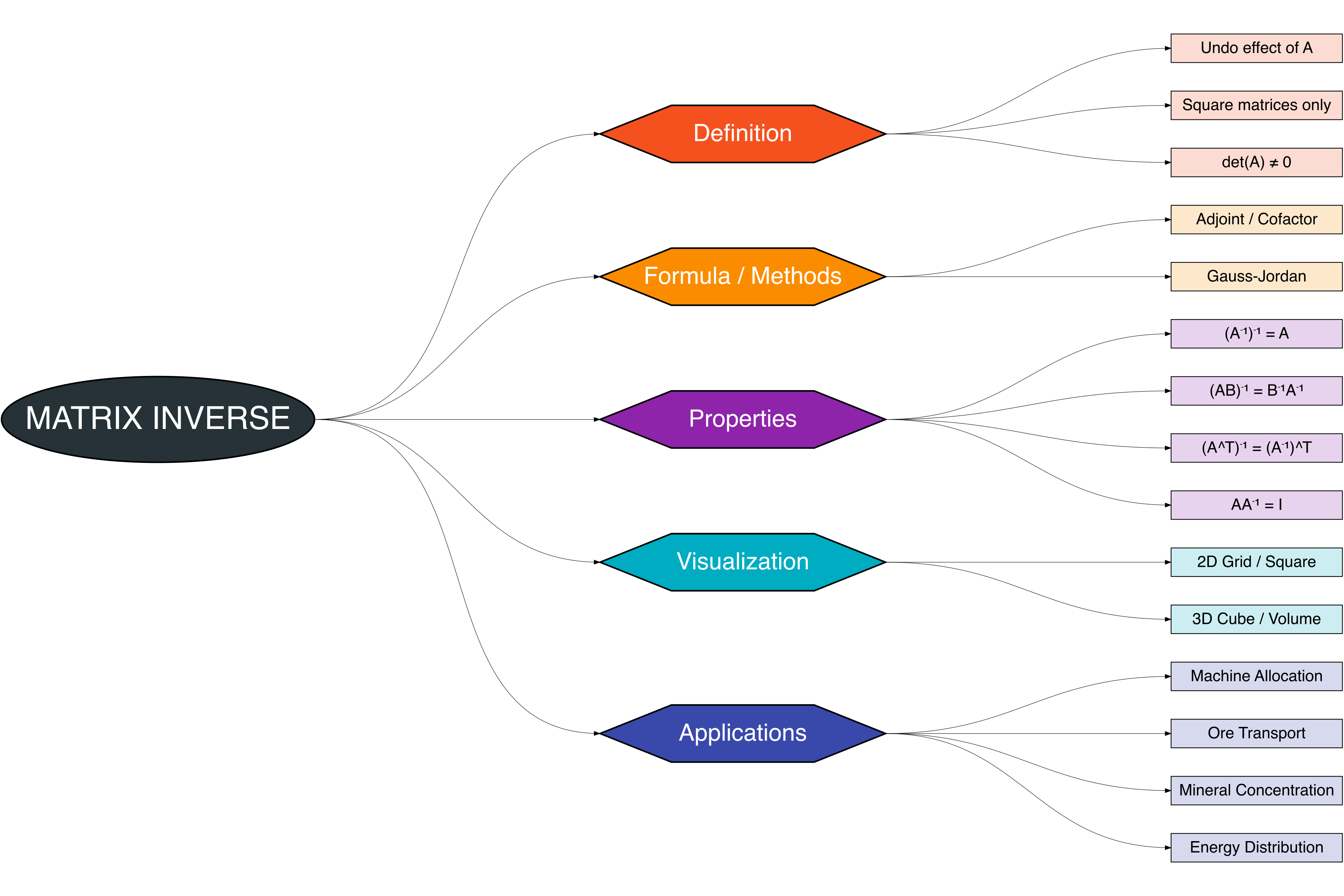
A Figure 3.1 provides a structured overview of the key topics discussed:
The matrix inverse is one of the most important concepts in linear algebra [1]–[3]. Think of it as the matrix version of division for numbers. Just like dividing a number \(b\) by \(a\) (where \(a \neq 0\)) gives \(x = b / a\), the matrix inverse allows us to “divide” by a matrix to solve equations. It is primarily used for solving systems of linear equations (SLE) [4], [5].
For example, if we have \(A \mathbf{x} = \mathbf{b}\) where \(A\) is a square matrix and \(\mathbf{b}\) is a column vector, the solution can be written as \(\mathbf{x} = A^{-1} \mathbf{b}.\) Here, \(A^{-1}\) is the inverse of matrix \(A\), which “undoes” the effect of \(A\) on \(\mathbf{x}\), similar to how \(1/a\) undoes multiplication by \(a\) for numbers [6], [7].
Key Notes:
- The inverse exists only for square matrices (\(n \times n\)). Rectangular matrices do not have inverses in the usual sense.
- Think of \(A^{-1}\) as the “undo button” for \(A\):
\[ A A^{-1} = A^{-1} A = I_n \]
where \(I_n\) is the identity matrix of size \(n \times n\). - If a matrix is singular (\(\det(A) = 0\)), the “undo button” does not exist.
3.1 Inverse Definition
A matrix \(B\) is called the inverse of a square matrix \(A\) if it satisfies:
\[ AB = BA = I_n \]
where \(I_n\) is the \(n \times n\) identity matrix.
- Notation: \(B = A^{-1}\)
- Existence condition: \(\det(A) \neq 0\)
- If \(\det(A) = 0\), then \(A\) is called a singular matrix, and the inverse does not exist.
The inverse of a matrix plays the role of “division” in linear algebra: it allows us to solve systems of linear equations efficiently by undoing the effect of multiplication by \(A\) [8], [9].
3.2 Inverse Formula
In linear algebra, several methods can be used to compute the inverse of a square matrix. One of the most classical and commonly taught approaches is the Adjoint (Cofactor) Method, which expresses the inverse in terms of the determinant and the adjoint of the matrix. This formula provides not only a theoretical foundation but also a practical way to compute inverses for small matrices.
3.2.1 Adjoint / Cofactor Method
For a square matrix \(A = [a_{ij}]_{n \times n}\), the inverse is given by:
\[ A^{-1} = \frac{1}{\det(A)} \, \text{adj}(A) \]
where \(\text{adj}(A)\) is the adjoint matrix, obtained by taking the transpose of the cofactor matrix of \(A\).
- Condition: \(\det(A) \neq 0\)
- If \(\det(A) = 0\), then \(A\) is not invertible (singular).
This method is practical for small matrices (e.g., \(2 \times 2\) or \(3 \times 3\)), but computationally expensive for large matrices, where Gaussian elimination or LU decomposition is preferred [1], [2], [5].
Note
Step 1: Adjoint (Adjugate) Matrix
The adjoint matrix \(\text{adj}(A)\) is defined as the transpose of the cofactor matrix:
\[ \text{adj}(A) = [C_{ji}] \]
This means:
- Compute all cofactors \(C_{ij}\)
- Then take the transpose to form \(\text{adj}(A)\).
Step 2 Cofactor
The cofactor \(C_{ij}\) is defined as:
\[ C_{ij} = (-1)^{i+j} \det(M_{ij}) \]
where \(M_{ij}\) is the minor of \(A\), obtained by removing the \(i\)-th row and the \(j\)-th column from \(A\).
- The factor \((-1)^{i+j}\) is called the cofactor sign.
- The cofactor signs follow a checkerboard pattern:
\[ \begin{bmatrix} + & - & + & - & \dots \\ - & + & - & + & \dots \\ + & - & + & - & \dots \\ - & + & - & + & \dots \\ \vdots & \vdots & \vdots & \vdots & \ddots \end{bmatrix} \]
Step 3 Steps to Compute \(A^{-1}\) using the Adjoint Method
- Compute the determinant \(\det(A)\). If \(\det(A) = 0\), stop (no inverse exists).
- Compute all minors \(M_{ij}\) for each element \(a_{ij}\).
- Compute the cofactors using:
\[ C_{ij} = (-1)^{i+j}\det(M_{ij}) \]
- Construct the cofactor matrix \(C = [C_{ij}]\).
- Transpose the cofactor matrix to get \(\text{adj}(A)\).
- Apply the formula:
\[ A^{-1} = \frac{1}{\det(A)} \, \text{adj}(A) \]
Example: 2D Matrix
\[ A = \begin{bmatrix} a & b \\ c & d \end{bmatrix} \]
- Determinant: \(\det(A) = ad - bc\)
- Cofactors:
- \(C_{11} = d\), \(C_{12} = -c\), \(C_{21} = -b\), \(C_{22} = a\)
Cofactor matrix: \[ C = \begin{bmatrix} d & -c \\ -b & a \end{bmatrix} \]
Adjoint: \[ \text{adj}(A) = \begin{bmatrix} d & -b \\ -c & a \end{bmatrix} \]
Thus: \[ A^{-1} = \frac{1}{ad - bc} \begin{bmatrix} d & -b \\ -c & a \end{bmatrix} \]
Example: 3D Matrix
\[ A = \begin{bmatrix} 1 & 2 & 3 \\ 0 & 4 & 5 \\ 1 & 0 & 6 \end{bmatrix} \]
- Determinant:
\[ \det(A) = 1(4 \cdot 6 - 5 \cdot 0) - 2(0 \cdot 6 - 5 \cdot 1) + 3(0 \cdot 0 - 4 \cdot 1) \]
\[ = 24 - (-10) - 12 = 22 \]
- Some cofactors:
- \(M_{11} = \begin{bmatrix} 4 & 5 \\ 0 & 6 \end{bmatrix}, \ \det(M_{11}) = 24 \implies C_{11} = +24\)
- \(M_{12} = \begin{bmatrix} 0 & 5 \\ 1 & 6 \end{bmatrix}, \ \det(M_{12}) = -5 \implies C_{12} = +5\)
- \(M_{13} = \begin{bmatrix} 0 & 4 \\ 1 & 0 \end{bmatrix}, \ \det(M_{13}) = -4 \implies C_{13} = -4\)
- \(M_{11} = \begin{bmatrix} 4 & 5 \\ 0 & 6 \end{bmatrix}, \ \det(M_{11}) = 24 \implies C_{11} = +24\)
(Continue this process for all \(C_{ij}\), then construct the cofactor matrix, transpose it, and finally compute \(A^{-1}\)).
Key Notes:
- The adjoint method is practical for small matrices (2×2, 3×3).
- For larger matrices, it is usually more efficient to use Gauss-Jordan elimination or other numerical methods.
3.2.2 Gauss-Jordan Method
The Gauss–Jordan method is one of the most systematic ways to compute the inverse of a square matrix.
Unlike the adjoint/cofactor method, it avoids computing determinants and cofactors, which can become tedious for larger matrices.
If \(A\) is an invertible \(n \times n\) matrix, then there exists \(A^{-1}\) such that:
\[ A A^{-1} = I_n \]
To find \(A^{-1}\), we apply row operations to reduce \(A\) to the identity matrix, while performing the same operations on \(I_n\).
The resulting right-hand side will then be \(A^{-1}\) [1], [2], [5].
Note:
Step 1: Form the Augmented Matrix
Construct the augmented matrix by placing the identity matrix \(I_n\) to the right of \(A\):
\[ [A \mid I_n] \]
This creates a block matrix with \(A\) on the left and \(I_n\) on the right.
Step 2: Apply Gauss–Jordan Elimination
Use elementary row operations to reduce the left block (\(A\)) into the identity matrix \(I_n\). At the same time, apply those same operations to the right block. The goal is to transform:
\[ [A \mid I_n] \quad \longrightarrow \quad [I_n \mid A^{-1}] \]
Step 3: Extract the Inverse
Once the left block is the identity matrix \(I_n\), the right block will be the inverse of \(A\):
\[ [A \mid I_n] \sim [I_n \mid A^{-1}] \]
Example:
Let \[ A = \begin{bmatrix} 2 & 1 \\ 5 & 3 \end{bmatrix} \] Step 1: Form the augmented matrix \[ [A \mid I_2] = \begin{bmatrix} 2 & 1 & \mid & 1 & 0 \\ 5 & 3 & \mid & 0 & 1 \end{bmatrix} \]
Step 2: Apply row operations
Make the pivot in the first row equal to 1:
\(R_1 \to \tfrac{1}{2} R_1\)
\[ \begin{bmatrix} 1 & 0.5 & \mid & 0.5 & 0 \\ 5 & 3 & \mid & 0 & 1 \end{bmatrix} \]Eliminate the 5 below the pivot:
\(R_2 \to R_2 - 5R_1\)
\[ \begin{bmatrix} 1 & 0.5 & \mid & 0.5 & 0 \\ 0 & 0.5 & \mid & -2.5 & 1 \end{bmatrix} \]Scale the second row to make the pivot 1:
\(R_2 \to 2R_2\)
\[ \begin{bmatrix} 1 & 0.5 & \mid & 0.5 & 0 \\ 0 & 1 & \mid & -5 & 2 \end{bmatrix} \]Eliminate the 0.5 above the pivot:
\(R_1 \to R_1 - 0.5R_2\)
\[ \begin{bmatrix} 1 & 0 & \mid & 3 & -1 \\ 0 & 1 & \mid & -5 & 2 \end{bmatrix} \]
Step 3: Extract the inverse \[ A^{-1} = \begin{bmatrix} 3 & -1 \\ -5 & 2 \end{bmatrix} \]
Key Notes:
- This method is highly effective for both hand calculations (small matrices) and computer algorithms (large matrices).
- If at any step a pivot element is \(0\), row exchanges may be needed.
- If the matrix cannot be reduced to \(I_n\), then \(A\) is singular and has no inverse.
3.3 Inverse Properties
The inverse of a matrix has several important properties that are fundamental in linear algebra.These properties describe how inverses behave under various operations such as taking another inverse, multiplying matrices, or transposing them. They also establish the necessary conditions for the existence of an inverse and its relation to the identity matrix [8]–[10].
- Inverse of inverse: \((A^{-1})^{-1} = A\)
- Inverse of product: \((AB)^{-1} = B^{-1} A^{-1}\)
- Inverse of transpose: \((A^T)^{-1} = (A^{-1})^T\)
- Existence: \(\det(A) \neq 0 \Rightarrow A^{-1}\) exists
- Non-existence: \(\det(A) = 0 \Rightarrow A^{-1}\) does not exist (singular)
- Identity relation: \(AA^{-1} = A^{-1}A = I_n\)
3.4 Inverse Visualizations
The matrix inverse can also be understood geometrically. An invertible matrix \(A\) represents a linear transformation in space. Its inverse \(A^{-1}\) reverses that transformation, mapping transformed points back to their original positions.
3.4.1 2D Matrix
The concept of a matrix inverse can be better understood in 2D using a unit square and its corner points. A \(2 \times 2\) matrix can be seen as a way to move points in the plane. The inverse matrix undoes that movement and brings the points back to their original positions.
Example
Imagine working with an underground mining survey grid:
Original Square:
The survey grid starts from \((0,0)\) with corners: \((0,0), (1,0), (0,1), (1,1)\). This represents an ideal survey map, perfectly aligned and scaled.After Matrix \(A\): Due to measurement errors in the field (e.g., compass deviation, magnetic interference, or narrow tunnel conditions), the survey grid may become skewed or distorted. The square then turns into a parallelogram. In practice, this is like a survey map drawn with errors in scale or orientation.
After \(A^{-1}\)
By applying the inverse matrix, the distorted data can be corrected. The parallelogram is restored back to the original square. This is similar to correcting a survey map so it matches the proper engineering coordinate system.
Key Notes:
- Matrix \(A\) = represents the distortion in the survey grid.
- Inverse Matrix \(A^{-1}\) = provides the correction that restores the map.
- Determinant \(\det(A)\) = shows whether the correction is possible.
- If \(\det(A) = 0\), the grid collapses into a line → information is lost → the map cannot be corrected.
Visualization
2D Matrix Inverse in Mining Grid
3.4.2 3D Matrix Inverse
A \(3 \times 3\) matrix in 3D space is closely related to the concept of volume and the existence of an inverse:
- If \(\det(A) \neq 0\), then \(A^{-1}\) exists.
- The determinant \(\det(A)\) gives the volume scaling factor.
- If \(\det(A) = 0\), the unit cube collapses into a lower dimension (a plane or a line) → no volume → no inverse.
- \(A^{-1}\) restores the cube to its original geometry.
Example
In mining engineering, this is important in block modeling:
- \(A\) modifies the unit cube (mining block).
- \(\det(A)\) indicates how much the ore volume is scaled.
- \(A^{-1}\) ensures we can recover the true geometry for accurate resource estimation.
\[ A = \begin{bmatrix} 1 & 2 & 0 \\ 0 & 1 & 3 \\ 2 & -1 & 1 \end{bmatrix}, \quad A^{-1} = \frac{1}{9} \begin{bmatrix} 4 & -2 & 6 \\ 6 & 1 & -3 \\ -2 & 2 & 1 \end{bmatrix} \]
Key Notes:
- \(\det(A) = 9 \;\;\Rightarrow\;\;\) volume scaled by factor \(9\).
- After \(A\): the original cube is transformed into a parallelepiped with 9 times the volume. This represents how a mining block might be distorted due to coordinate transformation or survey error.
- After \(A^{-1}\): the parallelepiped is transformed back into the original cube, ensuring that the true block geometry is recovered for accurate mine planning and resource estimation.
Visualization
Transformation by A and A⁻¹ on a Unit Cube
3.5 Applied of Invers
Here are some example problems showing applications of matrix inversion in mining operations.
3.5.1 Mining Equipment Allocation
A mine has three types of machines: Excavator (E), Dump Truck (D), and Conveyor (C). Each machine produces a certain output per hour:
| Machine | Ore (ton) | Waste (ton) | Energy (kWh) |
|---|---|---|---|
| E | 5 | 2 | 10 |
| D | 2 | 3 | 5 |
| C | 1 | 0 | 3 |
If the total ore, waste, and energy required per hour are:
\[ \text{Ore} = 20, \quad \text{Waste} = 15, \quad \text{Energy} = 50 \]
Determine the number of machines of each type needed using inverse matrix.
3.5.2 Ore Transport System
Three locations in a mine have different transport capacities and interdependencies:
\[ \begin{cases} x_1 + 2x_2 + x_3 = 100 \\ 2x_1 + x_2 + 3x_3 = 150 \\ x_1 + x_2 + 2x_3 = 120 \end{cases} \]
- \(x_1, x_2, x_3\) = number of trucks used on routes 1, 2, and 3.
Use inverse matrix to determine \(x_1, x_2, x_3\).
3.5.3 Mineral Concentration Modeling
A mineral separation process produces three by-products: A, B, C. The relationship between raw material and products is:
\[ \begin{bmatrix} 2 & 1 & 1 \\ 1 & 3 & 2 \\ 1 & 2 & 2 \end{bmatrix} \begin{bmatrix} x_1 \\ x_2 \\ x_3 \end{bmatrix} = \begin{bmatrix} 100 \\ 150 \\ 120 \end{bmatrix} \]
Calculate \(x_1, x_2, x_3\) = raw materials used per hour using \(A^{-1}\).
3.5.4 Energy Distribution
A mine has three sectors: Excavation, Transportation, and Processing. Energy (kWh) required in each sector depends on the number of machine units:
\[ \begin{bmatrix} 3 & 1 & 2 \\ 2 & 4 & 1 \\ 1 & 1 & 3 \end{bmatrix} \begin{bmatrix} x_1 \\ x_2 \\ x_3 \end{bmatrix} = \begin{bmatrix} 60 \\ 70 \\ 50 \end{bmatrix} \]
Use inverse matrix to find the optimal machine distribution \(x_1, x_2, x_3\).
Refrences
[1]
Lay, D. C., Linear algebra and its applications, Pearson, 2012
[2]
Strang, G., Introduction to linear algebra, Wellesley-Cambridge Press, Wellesley, MA, 2016
[3]
Anton, H., Elementary linear algebra, Wiley, New York, NY, 2013
[4]
Meyer, C. D., Matrix analysis and applied linear algebra, SIAM, 2000
[5]
Golub, G. H. and Loan, C. F. V., Matrix computations, Johns Hopkins University Press, Baltimore, MD, 2013
[6]
Trefethen, L. N. and David Bau, I., Numerical linear algebra, SIAM, 1997
[7]
Saikia, S., Recent advances in linear algebra applications, Linear Algebra and Its Applications, vol. 591, 123–145, 2020
[8]
OpenAI, ChatGPT conversation reference 0, Generated AI reference, 2025
[9]
OpenAI, ChatGPT conversation reference 1, Generated AI reference, 2025
[10]
OpenAI, ChatGPT conversation reference 2, Generated AI reference, 2025