4 Matrix Factorization
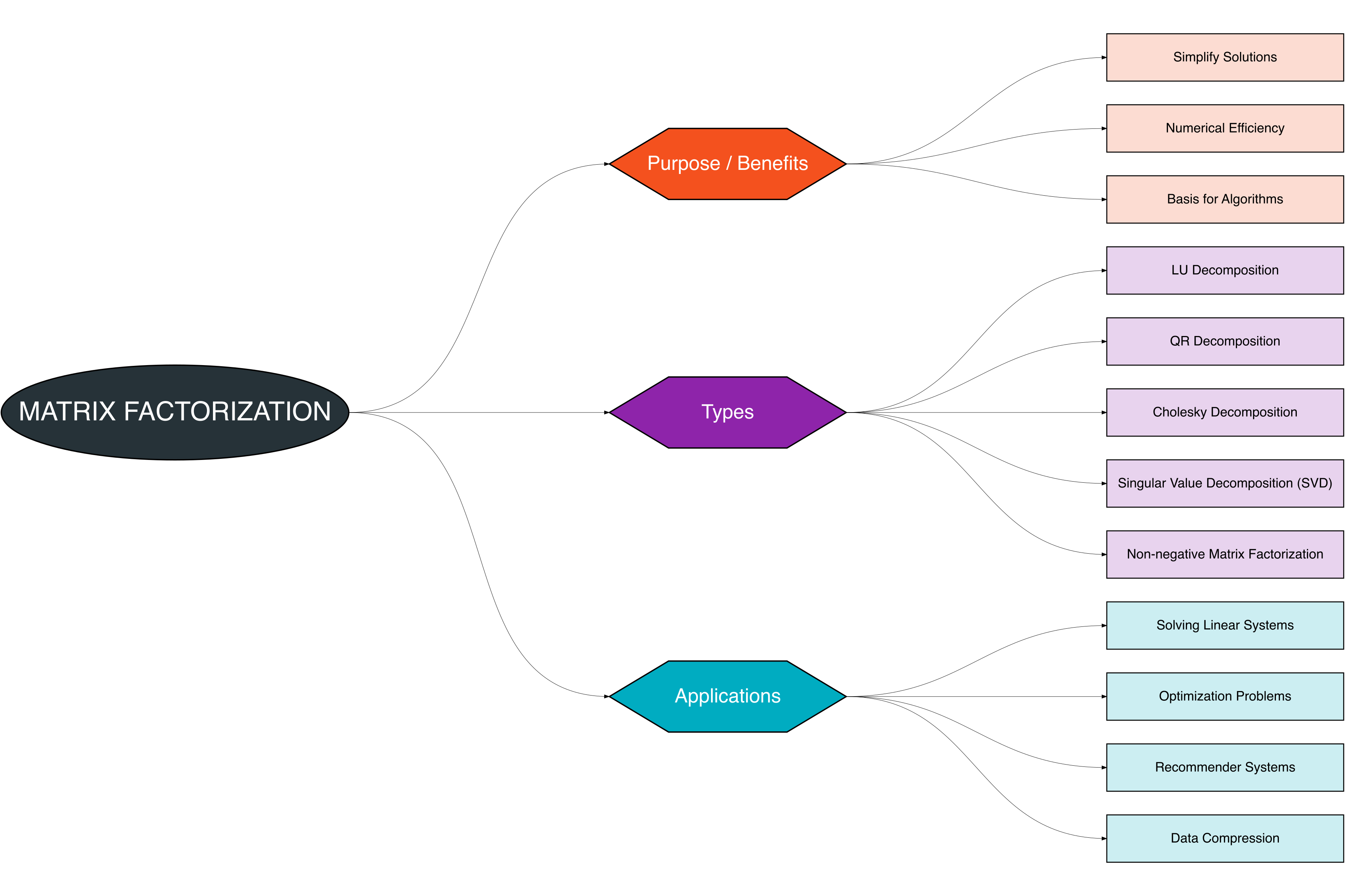
In this chapter, we explore the concept of matrix factorization and its applications. A Figure 4.1 provides a structured overview of the key topics discussed:
Matrix factorization is a powerful tool in linear algebra that decomposes a matrix into a product of two or more matrices. It is widely used in solving linear systems, numerical algorithms, optimization, and data analysis [1], [2].
4.1 Purpose / Benefits
Matrix factorization is useful for several reasons, particularly in simplifying computations and supporting advanced methods in linear algebra.
| Reason | Description |
|---|---|
| Simplify Solutions | Decomposing a matrix into simpler matrices can make solving linear systems faster and easier. |
| Numerical Efficiency | Factorization allows for stable and efficient computations, especially for large matrices. |
| Basis for Algorithms | Many advanced algorithms in numerical linear algebra rely on matrix factorization as a foundation. |
4.2 Types of Matrix Factorization
Several types of matrix factorizations are commonly used:
4.2.1 LU Decomposition
- Decomposes a square matrix \(A\) into a product of a lower triangular matrix \(L\) and an upper triangular matrix \(U\):
\[ A = LU \] - Useful for solving linear systems and inverting matrices efficiently.
4.2.2 QR Decomposition
- Decomposes a matrix \(A\) into an orthogonal matrix \(Q\) and an upper triangular matrix \(R\):
\[ A = QR \] - Often used in least squares problems and eigenvalue computations.
4.2.3 Cholesky Decomposition
- Applicable to symmetric, positive-definite matrices.
- Decomposes \(A\) as:
\[ A = LL^T \] where \(L\) is a lower triangular matrix.
- Common in optimization and numerical simulations.
4.2.4 Singular Value Decomposition
- Any \(m \times n\) matrix \(A\) can be decomposed as:
\[ A = U \Sigma V^T \] where \(U\) and \(V\) are orthogonal matrices and \(\Sigma\) is diagonal with singular values.
- Widely used in data compression, dimensionality reduction, and recommender systems.
4.2.5 Non-negative Matrix Factorization
- Decomposes a matrix \(A\) into matrices \(W\) and \(H\) with non-negative entries:
\[ A \approx WH \] - Used in feature extraction, text mining, and image processing.
4.3 Applications
Matrix factorization has diverse applications across engineering, data science, and applied mathematics. The table below summarizes key use cases:
| Application Area | Description | Methods Commonly Used |
|---|---|---|
| Solving Linear Systems | Factorizations such as LU or Cholesky allow faster and more stable solutions to \(Ax = b\). | LU, Cholesky |
| Optimization Problems | Many optimization algorithms rely on matrix factorizations to improve computational efficiency. | QR, Cholesky |
| Recommender Systems | SVD and NMF are used in collaborative filtering for predicting user preferences. | SVD, NMF |
| Data Compression | SVD reduces dimensionality of data while preserving essential structure, widely used in image and signal processing. | SVD |
4.3.1 Solving Linear Systems with LU
Suppose we have a linear system:
\[ A x = b, \quad A = \begin{bmatrix} 2 & 1 & 1 \\ 4 & -6 & 0 \\ -2 & 7 & 2 \end{bmatrix}, \quad b = \begin{bmatrix} 5 \\ -2 \\ 9 \end{bmatrix}, \quad x = \begin{bmatrix} x_1 \\ x_2 \\ x_3 \end{bmatrix} \]
LU decomposition:
\[ A = LU = \begin{bmatrix} 1 & 0 & 0 \\ 2 & 1 & 0 \\ -1 & -1 & 1 \end{bmatrix} \begin{bmatrix} 2 & 1 & 1 \\ 0 & -8 & -2 \\ 0 & 0 & 3 \end{bmatrix} \]
Solve in two steps:
- Forward substitution \(Ly = b\):
\[ \begin{bmatrix} 1 & 0 & 0 \\ 2 & 1 & 0 \\ -1 & -1 & 1 \end{bmatrix} \begin{bmatrix} y_1 \\ y_2 \\ y_3 \end{bmatrix} = \begin{bmatrix} 5 \\ -2 \\ 9 \end{bmatrix} \implies y_1 = 5, \ y_2 = -12, \ y_3 = 16 \]
- Backward substitution \(Ux = y\):
\[ \begin{bmatrix} 2 & 1 & 1 \\ 0 & -8 & -2 \\ 0 & 0 & 3 \end{bmatrix} \begin{bmatrix} x_1 \\ x_2 \\ x_3 \end{bmatrix} = \begin{bmatrix} 5 \\ -12 \\ 16 \end{bmatrix} \implies x_3 = \frac{16}{3}, \ x_2 = \frac{1}{6}, \ x_1 = \frac{11}{12} \]
Solution:
\[ x = \begin{bmatrix} x_1 \\ x_2 \\ x_3 \end{bmatrix} = \begin{bmatrix} \frac{11}{12} \\ \frac{1}{6} \\ \frac{16}{3} \end{bmatrix} \]
4.3.2 Optimization Problems
Matrix factorization is widely used in optimization to improve computational efficiency and simplify complex calculations. Many optimization algorithms require solving linear systems or decomposing matrices multiple times, and factorization helps speed up these computations.
Example: Quadratic Optimization Problem
Suppose we want to minimize a quadratic function:
\[ f(x) = \frac{1}{2} x^T Q x - b^T x \]
where \(Q\) is a symmetric positive definite matrix, \(b\) is a vector, and \(x\) is the variable vector:
\[ Q = \begin{bmatrix} 4 & 2 & 0 \\ 2 & 5 & 1 \\ 0 & 1 & 3 \end{bmatrix}, \quad b = \begin{bmatrix} 2 \\ -1 \\ 3 \end{bmatrix}, \quad x = \begin{bmatrix} x_1 \\ x_2 \\ x_3 \end{bmatrix} \]
Step 1: Factorize \(Q\) using Cholesky decomposition
Since \(Q\) is symmetric positive definite:
\[ Q = LL^T, \quad L = \begin{bmatrix} 2 & 0 & 0 \\ 1 & 2 & 0 \\ 0 & 0.5 & \sqrt{2.75} \end{bmatrix} \]
Step 2: Solve \(Q x = b\) using forward and backward substitution
- Forward substitution: \(Ly = b\)
\[ \begin{bmatrix} 2 & 0 & 0 \\ 1 & 2 & 0 \\ 0 & 0.5 & \sqrt{2.75} \end{bmatrix} \begin{bmatrix} y_1 \\ y_2 \\ y_3 \end{bmatrix} = \begin{bmatrix} 2 \\ -1 \\ 3 \end{bmatrix} \implies y_1 = 1, \ y_2 = -1.5, \ y_3 \approx 2.70 \]
- Backward substitution: \(L^T x = y\)
\[ \begin{bmatrix} 2 & 1 & 0 \\ 0 & 2 & 0.5 \\ 0 & 0 & \sqrt{2.75} \end{bmatrix} \begin{bmatrix} x_1 \\ x_2 \\ x_3 \end{bmatrix} = \begin{bmatrix} 1 \\ -1.5 \\ 2.70 \end{bmatrix} \implies x_3 \approx 1.63, \ x_2 \approx -1.92, \ x_1 \approx 1.46 \]
Solution:
\[ x \approx \begin{bmatrix} 1.46 \\ -1.92 \\ 1.63 \end{bmatrix} \]
Key Takeaways:
- Factorization (like LU or Cholesky) allows efficient repeated solutions when \(Q\) changes slightly, common in iterative optimization.
- Reduces computational cost from \(O(n^3)\) to roughly \(O(n^2)\) per solve in large systems.
- Ensures numerical stability, critical in sensitive optimization problems.
4.3.3 Recommender Systems
Matrix factorization plays a crucial role in collaborative filtering, which is widely used in recommender systems to predict user preferences based on historical data.
Problem Setup: User-Item Ratings
Suppose we have a user-item rating matrix \(R\):
\[ R = \begin{bmatrix} 5 & 3 & 0 & 1 \\ 4 & 0 & 0 & 1 \\ 1 & 1 & 0 & 5 \\ 0 & 0 & 5 & 4 \end{bmatrix} \]
- Rows represent users (\(u_1, u_2, u_3, u_4\))
- Columns represent items (\(i_1, i_2, i_3, i_4\))
- A value of 0 indicates a missing rating.
Step 1: Factorize \(R\) using low-rank approximation
We approximate \(R\) by the product of two smaller matrices:
\[ R \approx U V^T \]
where:
- \(U \in \mathbb{R}^{4 \times 2}\) represents user features
- \(V \in \mathbb{R}^{4 \times 2}\) represents item features
Example:
\[ U = \begin{bmatrix} 1 & 0.5 \\ 0.9 & 0.4 \\ 0.2 & 1 \\ 0.1 & 0.9 \end{bmatrix}, \quad V = \begin{bmatrix} 1 & 0.3 \\ 0.8 & 0.5 \\ 0.2 & 1 \\ 0.5 & 0.7 \end{bmatrix} \]
Step 2: Predict missing ratings
The predicted rating for user \(u_i\) and item \(i_j\) is:
\[ \hat{R}_{ij} = U_i \cdot V_j^T \]
Example: Predict the missing rating for \(u_1\) on item \(i_3\):
\[ \hat{R}_{13} = [1, 0.5] \cdot [0.2, 1]^T = 1*0.2 + 0.5*1 = 0.7 \]
Step 3: Recommendation
- Recommend items with highest predicted ratings for each user.
- Helps in personalized suggestions even with sparse data.
Key Takeaways:
- SVD or NMF (Non-negative Matrix Factorization) are common factorization methods.
- Reduces dimensionality of the rating matrix while capturing latent user and item features.
- Enables scalable and accurate recommendations for large datasets.
4.3.4 Data Compression
Matrix factorization is widely used in data compression to reduce the dimensionality of datasets while retaining important structure. This is especially common in images, videos, and signals.
Problem Setup: Image as a Matrix
Suppose we have a grayscale image represented as a matrix \(A\):
\[ A = \begin{bmatrix} 255 & 200 & 180 \\ 240 & 190 & 170 \\ 230 & 180 & 160 \end{bmatrix} \]
Each entry represents the intensity of a pixel (0 = black, 255 = white).
Step 1: Apply Singular Value Decomposition (SVD)
We factorize \(A\) into three matrices:
\[ A = U \Sigma V^T \]
where:
- \(U\) contains left singular vectors (features of rows)
- \(\Sigma\) is a diagonal matrix with singular values (importance of features)
- \(V^T\) contains right singular vectors (features of columns)
Example:
\[ \Sigma = \begin{bmatrix} 600 & 0 & 0 \\ 0 & 50 & 0 \\ 0 & 0 & 10 \end{bmatrix} \]
Step 2: Reduce Rank for Compression
Keep only the largest \(k\) singular values (rank-\(k\) approximation):
\[ A_k = U_k \Sigma_k V_k^T \]
For example, keeping \(k=2\) largest singular values:
\[ \Sigma_2 = \begin{bmatrix} 600 & 0 \\ 0 & 50 \end{bmatrix} \]
Step 3: Reconstruct Compressed Data
The compressed matrix \(A_2\) approximates \(A\) with fewer data:
\[ A_2 \approx \begin{bmatrix} 254 & 199 & 179 \\ 239 & 189 & 169 \\ 231 & 181 & 161 \end{bmatrix} \]
- Notice that the image is almost identical but requires less storage.
- Compression ratio improves as \(k\) decreases.
Key Takeaways:
- SVD is effective for low-rank approximation and noise reduction.
- Useful in image compression, signal processing, and dimensionality reduction.
- Retains the most important features while discarding less significant information.
Refrences
[1]
Meyer, C. D., Matrix analysis and applied linear algebra, SIAM, 2000
[2]
Golub, G. H. and Loan, C. F. V., Matrix computations, Johns Hopkins University Press, Baltimore, MD, 2013