2 Data Exploration
After understanding the important role of statistics in turning raw data into meaningful insights as mentioned in chapter Intro to Statistics, the next step is to explore the nature of data and how it can be classified. Data forms the foundation of any analysis, and without a clear understanding of its types and structure, organizing, interpreting, and making accurate decisions can be challenging [1].
This section provides a Data Exploration Figure 2.1, covering the classification of data into numeric (quantitative) and categorical (qualitative) types, including subtypes such as discrete, continuous, nominal, and ordinal [2]. It also discusses data sources and the basic structure of a dataset, including variables and observations [3]. By mastering these concepts, readers will gain a solid foundation for subsequent analytical steps and will be better equipped to recognize and handle different forms of data in context [4]–[8].
2.1 Types of Data
In statistics, understanding the types of data is a crucial starting point. Data can be broadly divided into two main groups: numerical and categorical. Numerical data represent numbers that can be either discrete (countable, such as the number of students) or continuous (measurable, such as height or temperature) [9]. Categorical data, on the other hand, represent labels or groups. They can be nominal (without order, such as gender or colors) or ordinal (with order, such as satisfaction levels: low, medium, high) [10].
Knowing the correct type of data is essential because it guides us in choosing the right statistical methods, the most suitable visualizations, and ensures that our interpretations are accurate [11]. The following video will help you clearly understand these concepts through simple explanations and real-world examples.
2.2 Numeric (Quantitativ)
Numeric or quantitative data are data expressed in numbers that represent counts or measurements[2]. They provide information about how much or how many of something, allowing for mathematical operations such as addition, subtraction, averaging, and statistical analysis [3].
Quantitative data are divided into two main types:
- Discrete data: consist of countable whole numbers (e.g., number of students, number of cars) [1].
- Continuous data: consist of measurable values that can take on decimals (e.g., height, weight, temperature) [2].
2.2.1 Discrete
Discrete data are numerical values that can be counted and usually take whole numbers [1], [2]. These data cannot contain fractions or decimals, since each value represents a complete count. Examples include the number of children in a family, the number of cars owned, or the number of accidents in a month [1].
children <- c(2, 3, 1, 4, 2, 3, 2, 5, 0, 2) # Discrete Data Example
children                                    # Print result (way 1)
print(children)                             # Print result (way 2)
table(children)                             # frequency distribution
mean(children)                              # average
# Basic Visual
barplot(table(children),
main="Number of Children",
col="lightblue")
2.2.2 Continuous
Continuous data are numerical values obtained through measurement and can include fractions or decimals [2], [3]. These values are not limited and can take on any value within a given range. Examples include height, weight, temperature, and rainfall [2].
# Continuous Data Example
height <- c(165.2, 170.5, 172.3, 168.8, 174.1,
            169.4, 171.7, 173.6, 175.2, 166.8)
summary(height)hist(height,
col="skyblue",
main="Height Distribution",
xlab="Height (cm)")
2.3 Categorical (Qualitative)
Categorical or qualitative data are data expressed in labels, names, or categories rather than numbers [2]. They describe qualities, attributes, or classifications that cannot be meaningfully measured with arithmetic operations like addition or subtraction.
Categorical data are divided into two main types:
- Nominal data: categories without any natural order or ranking (e.g., gender, blood type, car brand) [1].
- Ordinal data: categories with a meaningful order or ranking, but without fixed differences between ranks (e.g., education level, satisfaction rating, socioeconomic status) [3].
2.3.1 Nominal
Nominal data are categorical values that act only as labels or identifiers, with no inherent order or ranking [1], [2]. They are used to classify objects into different groups, but there is no meaning of greater or lesser among the categories. Examples include gender, blood type, and product brands.
# Nominal Data Example
gender <- c("Male", "Female", "Male", "Male", "Female", "Female",
            "Male", "Female", "Male", "Female")
table(gender)barplot(table(gender),
col=c("pink","lightblue"),
main="Gender Distribution",
ylab="Count")
2.3.2 Ordinal
Ordinal data are categorical values that have a clear order or ranking, but the distance between categories is not precisely measurable [2]. These data show levels or rankings but do not indicate the magnitude of differences between them. Examples include satisfaction levels (low, medium, high), education levels, or competition rankings [2].
# Ordinal Data Example
satisfaction <- factor(c("Low","Medium","High","Medium","High","Low",
                         "Medium","High","Medium","Low"),
                       levels = c("Low","Medium","High"), ordered = TRUE)

table(satisfaction)barplot(table(satisfaction),
col=c("red","orange","green"),
main="Satisfaction Level",
ylab="Count")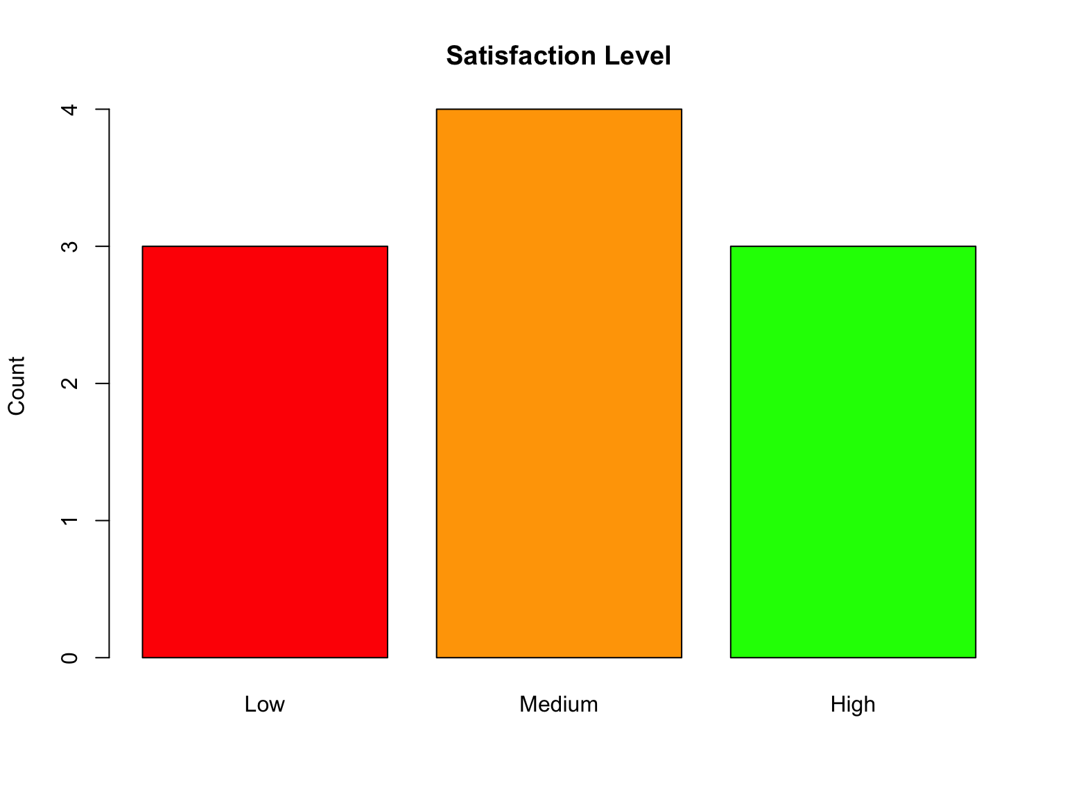
2.4 Data Sources
Data Sources are the origins of data used for analysis. Knowing the source is important because it affects data quality, validity, and relevance [12].
Types of Data Sources:
- Internal Sources – Data coming from within the organization, e.g., sales transactions, inventory records, financial reports, or employee data [13].
- External Sources – Data obtained from outside the organization, e.g., government statistics, industry reports, public datasets, social media, or third-party providers [13].
- Structured vs Unstructured Data
Consider the the following Video to know more about Structured and Unstructured Data!.
2.5 Data Structure
Data Structure refers to the way data is organized to make analysis easier and more efficient. A well-structured dataset helps with cleaning, processing, analyzing, and visualizing data [12]; [13]. The main components of data structure are:
- Dataset: A collection of data arranged in a structured format, usually as a table.
- Columns: Each column represents a variable or attribute describing the observations.
- Rows: Each row represents a single observation or case.
2.5.1 Dataset (Data Frame)
Example: An online store wants to analyze its sales performance over the first week of October 2025. They collect the following information for each transaction:
| Column | Type | Description |
|---|---|---|
| Date | Date | The date of the transaction |
| Qty | Discrete | The quantity sold (countable numbers) |
| Price | Continuous | The price per unit (decimal values allowed) |
| Product | Nominal | The product sold (categorical, no order) |
| CustomerTier | Ordinal | Customer tier: Low, Medium, High (ordered) |
# Create the example dataset
sales_data <- data.frame(
  Date = as.Date(c('2025-10-01', '2025-10-01', '2025-10-02', '2025-10-02')),
  Qty = c(2, 5, 1, 3),                                        # Discrete
  Price = c(1000, 20, 1000, 30),                              # Continuous
  Product = c('Laptop', 'Mouse', 'Laptop', 'Keyboard'),       # Nominal
  CustomerTier = factor(c('High', 'Medium', 'Low', 'Medium'), # Ordinal
                        levels = c('Low', 'Medium', 'High'),
                        ordered = TRUE))

print(sales_data)      # View the dataset / str(sales_data).
2.5.2 Variables (Columns)
Variables are the columns or attributes in a dataset that store specific pieces of information about each observation. They define what kind of data is collected and determine the types of analysis that can be performed [12].
2.5.3 Observations (Rows)
Observations are the rows in a dataset, with each row representing a single case, event, or unit of analysis [12]. Together, variables and observations form the core structure of a dataset, allowing us to organize, explore, and analyze data effectively [12].
References
[1]
Baker, L., Data types: Getting started with statistics, Everand, 2020, Available. https://www.everand.com/book/486797108/Data-Types-Getting-Started-With-Statistics
[2]
Shreffler, J., Types of variables and commonly used statistical designs, NCBI Bookshelf, 2023, Available. https://www.ncbi.nlm.nih.gov/books/NBK557882/
[3]
Baley, I. and Veldkamp, L., The data economy: Tools and applications, Princeton University Press, 2025, Available. https://press.princeton.edu/books/hardcover/9780691256726/the-data-economy
[4]
MyGreatLearning, 4 types of data - nominal, ordinal, discrete, continuous, Available. https://www.mygreatlearning.com/blog/types-of-data/
[5]
Canada, S., 4.2 types of variables, 2021, Available. https://www150.statcan.gc.ca/n1/edu/power-pouvoir/ch8/5214817-eng.htm
[6]
Adelaide, U. of, Types of data in statistics: Numerical vs categorical data, Available. https://online.adelaide.edu.au/blog/types-of-data
[7]
Scribbr, Types of variables in research & statistics | examples, 2022, Available. https://www.scribbr.com/methodology/types-of-variables/
[8]
GeeksforGeeks, Data types in statistics, 2025, Available. https://www.geeksforgeeks.org/maths/data-types-in-statistics/
[9]
James, G., Witten, D., Hastie, T., and Tibshirani, R., An introduction to statistical learning: With applications in r, Springer, 2021
[10]
Wakeling, I., Statistics in r using RStudio: An introduction for food scientists, Elsevier, Cambridge, MA, 2020
[11]
Hastie, T., Tibshirani, R., and Friedman, J., The elements of statistical learning: Data mining, inference, and prediction, Springer, 2021
[12]
Wickham, H., Tidy data: A practical guide to organizing and managing data in r, O’Reilly Media, Sebastopol, CA, 2023
[13]
Kelleher, J. D. and Tierney, B., Data science: An introduction, CRC Press, Boca Raton, FL, 2015