Chapter 6 Flow Control

suppressPackageStartupMessages({
  library(tidyverse, quietly = TRUE)   # loading ggplot2 and dplyr
})

As always, there is a Video Lecture that accompanies this chapter.

Often it is necessary to write scripts that perform different action depending on the data or to automate a task that must be repeated many times. To address these issues we will introduce the if statement and its closely related cousin if else. To address repeated tasks we will define two types of loops, a while loop and a for loop.

6.1 Logical Expressions

The most common logical expressions are the numerical expressions <, <=, ==, !=, >=, >. These are the usual logical comparisons from mathematics, with != being the not equal comparison. For any logical value or vector of values, the ! flips the logical values.

df <- data.frame(A=1:6, B=5:10)
df

##   A  B
## 1 1  5
## 2 2  6
## 3 3  7
## 4 4  8
## 5 5  9
## 6 6 10

df %>% mutate(`A==3?`         =  A == 3,
              `A<=3?`         =  A <= 3,
              `A!=3?`         =  A != 3,
              `Flip Previous` = ! `A!=3?` )

##   A  B A==3? A<=3? A!=3? Flip Previous
## 1 1  5 FALSE  TRUE  TRUE         FALSE
## 2 2  6 FALSE  TRUE  TRUE         FALSE
## 3 3  7  TRUE  TRUE FALSE          TRUE
## 4 4  8 FALSE FALSE  TRUE         FALSE
## 5 5  9 FALSE FALSE  TRUE         FALSE
## 6 6 10 FALSE FALSE  TRUE         FALSE

I find that it is preferable to write logical comparisons using < or <= rather than the “greater than” versions because the number line is read left to right, so it is much easier to have the smaller value on the left.

df %>% mutate( `A < B`  =  A < B)

##   A  B A < B
## 1 1  5  TRUE
## 2 2  6  TRUE
## 3 3  7  TRUE
## 4 4  8  TRUE
## 5 5  9  TRUE
## 6 6 10  TRUE

If we have two (or more) vectors of logical values, we can do two pairwise operations. The “and” operator & will result in a TRUE value if all elements are TRUE. The “or” operator will result in a TRUE value if either the left hand side or right hand side is TRUE.

df %>% mutate(C = A>=0,  D = A<=5) %>%
  mutate( result1_and = C & D,          #    C and D both true
          result2_and =  A>=0 & A<=5,   #    directly calculated
          result3_and =  0 <= A & A<=5, #    more readable 0 <= A <= 5
          result4_or  =  A<=0 | 5<=A)   #    A not in (0,5) range

##   A  B    C     D result1_and result2_and result3_and result4_or
## 1 1  5 TRUE  TRUE        TRUE        TRUE        TRUE      FALSE
## 2 2  6 TRUE  TRUE        TRUE        TRUE        TRUE      FALSE
## 3 3  7 TRUE  TRUE        TRUE        TRUE        TRUE      FALSE
## 4 4  8 TRUE  TRUE        TRUE        TRUE        TRUE      FALSE
## 5 5  9 TRUE  TRUE        TRUE        TRUE        TRUE       TRUE
## 6 6 10 TRUE FALSE       FALSE       FALSE       FALSE       TRUE

Next we can summarize a vector of logical values using any(), all(), and which(). These functions do exactly what you would expect them to do.

any(6:10 <= 7 )   # Should return TRUE because there are two TRUE results

## [1] TRUE

all(6:10 <= 7 )   # Should return FALSE because there is at least one FALSE result

## [1] FALSE

which( 6:10 <= 7) # return the indices of the TRUE values

## [1] 1 2

Finally, I often need to figure out if a character string is in some set of values.

df <- data.frame( Type = rep(c('A','B','C','D'), each=2), Value=rnorm(8) )
df

##   Type       Value
## 1    A  0.59402990
## 2    A  0.05041084
## 3    B  0.61352322
## 4    B  0.37585796
## 5    C  1.59620506
## 6    C -1.15972350
## 7    D  0.52400185
## 8    D -0.47470014

# df %>% filter( Type == 'A' | Type == 'B' )
df %>% filter( Type %in% c('A','B') )   # Only rows with Type == 'A' or Type =='B'

##   Type      Value
## 1    A 0.59402990
## 2    A 0.05041084
## 3    B 0.61352322
## 4    B 0.37585796

6.2 Decision statements

6.2.1 In `dplyr` wrangling

A very common task within a data wrangling pipeline is to create a new column that recodes information in another column. Consider the following data frame that has name, gender, and political party affiliation of six individuals. In this example, we’ve coded male/female as 1/0 and political party as 1,2,3 for democratic, republican, and independent.

people <- data.frame(
  name = c('Barack','Michelle', 'George', 'Laura', 'Bernie', 'Deborah'),
  gender = c(1,0,1,0,1,0),
  party = c(1,1,2,2,3,3)
)
people

##       name gender party
## 1   Barack      1     1
## 2 Michelle      0     1
## 3   George      1     2
## 4    Laura      0     2
## 5   Bernie      1     3
## 6  Deborah      0     3

The command ifelse() works quite well within a dplyr::mutate() command and it responds correctly to vectors. The syntax is ifelse( logical.expression, TrueValue, FalseValue ). The return object of this function is a vector that is appropriately made up of the TRUE and FALSE results.

For example, there we take the column gender and for each row test to see if the value is 0. If it is, the resulting element is Female otherwise it is Male.

people <- people %>%
  mutate( gender2 = ifelse( gender == 0, 'Female', 'Male') )
people

##       name gender party gender2
## 1   Barack      1     1    Male
## 2 Michelle      0     1  Female
## 3   George      1     2    Male
## 4    Laura      0     2  Female
## 5   Bernie      1     3    Male
## 6  Deborah      0     3  Female

To do something similar for the case where we have 3 or more categories, we could use the ifelse() command repeatedly to address each category level separately. However because the ifelse command is limited to just two cases, it would be nice if there was a generalization to multiple categories. The
dplyr::case_when function is that generalization. The syntax is case_when( logicalExpression1~Value1, logicalExpression2~Value2, ... ). We can have as many LogicalExpression ~ Value pairs as we want.

people <- people %>%
  mutate( party2 = case_when( party == 1 ~ 'Democratic', 
                              party == 2 ~ 'Republican', 
                              party == 3 ~ 'Independent',
                              TRUE       ~ 'None Stated' ) )
people

##       name gender party gender2      party2
## 1   Barack      1     1    Male  Democratic
## 2 Michelle      0     1  Female  Democratic
## 3   George      1     2    Male  Republican
## 4    Laura      0     2  Female  Republican
## 5   Bernie      1     3    Male Independent
## 6  Deborah      0     3  Female Independent

Often the last case is a catch all case where the logical expression will ALWAYS evaluate to TRUE and this is the value for all other input.

As another alternative to the problem of recoding factor levels, we could use the command forcats::fct_recode() function. See the Factors chapter in this book for more information about factors.

6.2.2 General `if else`

While programming, I often need to perform expressions that are more complicated than what the ifelse() command can do. Remember, the ifelse() command only can produce a vector. For any logic that is more complected that simply producing an output vector, we’ll need a more flexible approach. The downside is that it is slightly more complicated to use and does not automatically handle vector inputs for the comparison.

The general format of an if or an if else is presented below:.

# Simplest version
if( logical.test ){ # The logical test must be a SINGLE TRUE/FALSE value
  expression        # The expression could be many lines of code
}

# Including the optional else
if( logical.test ){
  expression
}else{
  expression
}

where the else part is optional.

Suppose that I have a piece of code that generates a random variable from the Binomial distribution with one sample (essentially just flipping a coin) but I’d like to label it head or tails instead of one or zero.

The test expression inside the if() is evaluated and if it is true, then the subsequent statement is executed. If the test expression is false, the next statement is skipped. The way the R language is defined, only the first statement after the if statement is executed (or skipped) depending on the test expression. If we want multiple statements to be executed (or skipped), we will wrap those expressions in curly brackets { }. I find it easier to follow the if else logic when I see the curly brackets so I use them even when there is only one expression to be executed. Also notice that the RStudio editor indents the code that might be skipped to try help give you a hint that it will be conditionally evaluated.

# Flip the coin, and we get a 0 or 1
result <- rbinom(n=1, size=1, prob=0.5)
result

## [1] 1

# convert the 0/1 to Tail/Head
if( result == 0 ){
  result <- 'Tail'
  print(" in the if statement, got a Tail! ")
}else{
  result <- 'Head'
  print("In the else part!") 
}

## [1] "In the else part!"

result

## [1] "Head"

Run this code several times until you get both cases several times. Notice that in the Environment tab in RStudio, the value of the variable result changes as you execute the code repeatedly.

To provide a more statistically interesting example of when we might use an if else statement, consider the calculation of a p-value in a 1-sample t-test with a two-sided alternative. Recall that the calculation was:

If the test statistic t is negative, then p-value = \(2*P\left(T_{df} \le t \right)\)
If the test statistic t is positive, then p-value = \(2*P\left(T_{df} \ge t \right)\).

# create some fake data
n  <- 20   # suppose this had a sample size of 20
x  <- rnorm(n, mean=2, sd=1)

# testing H0: mu = 0  vs Ha: mu =/= 0
t  <- ( mean(x) - 0 ) / ( sd(x)/sqrt(n) )
df <- n-1
if( t < 0 ){
  p.value <- 2 * pt(t, df)
}else{
  p.value <- 2 * (1 - pt(t, df))
}

# print the resulting p-value
p.value

## [1] 4.458162e-08

This sort of logic is necessary for the calculation of p-values and so something similar is found somewhere inside the t.test() function.

Finally we can nest if else statements together to allow you to write code that has many different execution routes.

# randomly grab a number between 0,5 and round it up to 1,2, ..., 5
birth.order <- ceiling( runif(1, 0,5) )  
if( birth.order == 1 ){
  print('The first child had more rules to follow')
}else if( birth.order == 2 ){
  print('The second child was ignored')
}else if( birth.order == 3 ){
  print('The third child was spoiled')
}else{
  # if birth.order is anything other than 1, 2 or 3
  print('No more unfounded generalizations!')
}

## [1] "The second child was ignored"

6.3 Loops

It is often desirable to write code that does the same thing over and over, relieving you of the burden of repetitive tasks. To do this we’ll need a way to tell the computer to repeat some section of code over and over. However we’ll usually want something small to change each time through the loop and some way to tell the computer how many times to run the loop or when to stop repeating.

6.3.1 `while` Loops

The basic form of a while loop is as follows:

# while loop with multiple lines to be repeated
while( logical.test ){
  expression1      # multiple lines of R code
  expression2
}

The computer will first evaluate the test expression. If it is true, it will execute the code once. It will then evaluate the test expression again to see if it is still true, and if so it will execute the code section a third time. The computer will continue with this process until the test expression finally evaluates as false.

x <- 1
while( x < 100 ){
  print( paste("In loop and x is now:", x) )  # print out current value of x
  x <- 2*x
}

## [1] "In loop and x is now: 1"
## [1] "In loop and x is now: 2"
## [1] "In loop and x is now: 4"
## [1] "In loop and x is now: 8"
## [1] "In loop and x is now: 16"
## [1] "In loop and x is now: 32"
## [1] "In loop and x is now: 64"

It is very common to forget to update the variable used in the test expression. In that case the test expression will never be false and the computer will never stop. This unfortunate situation is called an infinite loop.

# Example of an infinite loop!  Do not Run!
x <- 1
while( x < 10 ){
  print(x)
}

6.3.2 `for` Loops

Often we know ahead of time exactly how many times we should go through the loop. We could use a while loop, but there is also a second construct called a for loop that is quite useful.

The format of a for loop is as follows:

for( index in vector ){
  expression1
  expression2
}

where the index variable will take on each value in vector in succession and the next statement will be evaluated. As always, the statement can be multiple statements wrapped in curly brackets {}.

for( i in 1:5 ){
  print( paste("In the loop and current value is i =", i) )
}

## [1] "In the loop and current value is i = 1"
## [1] "In the loop and current value is i = 2"
## [1] "In the loop and current value is i = 3"
## [1] "In the loop and current value is i = 4"
## [1] "In the loop and current value is i = 5"

What is happening is that i starts out as the first element of the vector c(1,2,3,4,5), in this case, i starts out as 1. After i is assigned, the statements in the curly brackets are then evaluated. Once we get to the end of those statements, i is reassigned to the next element of the vector c(1,2,3,4,5). This process is repeated until i has been assigned to each element of the given vector. It is somewhat traditional to use i and j and the index variables, but they could be anything.

While the recipe above is the minimal definition of a for loop, there is often a bit more set up to create a result vector or data frame that will store the steps of the for loop.

N <- 10 
result <- NULL     # Make a place to store each step of the for loop
for( i in 1:N ){
  # Perhaps some code that calculates something
  result[i] <-  # something 
}

We can use this loop to calculate the first \(10\) elements of the Fibonacci sequence. Recall that the Fibonacci sequence is defined by \(F_{i}=F_{i-1}+F_{i-2}\) where \(F_{1}=0\) and \(F_{2}=1\).

N <- 10                # How many Fibonacci numbers to create
F <- rep(0,2)         # initialize a vector of zeros
F[1] <- 0              # F[1]  should be zero
F[2] <- 1              # F[2]  should be 1
print(F)               # Show the value of F before the loop

## [1] 0 1

for( i in 3:N ){
  F[i] <- F[i-1] + F[i-2] # define based on the prior two values
  print(F)                # show F at each step of the loop
}

## [1] 0 1 1
## [1] 0 1 1 2
## [1] 0 1 1 2 3
## [1] 0 1 1 2 3 5
## [1] 0 1 1 2 3 5 8
## [1]  0  1  1  2  3  5  8 13
## [1]  0  1  1  2  3  5  8 13 21
##  [1]  0  1  1  2  3  5  8 13 21 34

For a more statistical case where we might want to perform a loop, we can consider the creation of the bootstrap estimate of a sampling distribution. The bootstrap distribution is created by repeatedly re-sampling with replacement from our original sample data, running the analysis for each re-sample, and then saving the statistic of interest.

library(dplyr)
library(ggplot2)

# bootstrap from the trees dataset.
SampDist <- data.frame(xbar=NULL) # Make a data frame to store the means 
for( i in 1:1000 ){
  ## Do some stuff
  boot.data <- trees %>% dplyr::sample_frac(replace=TRUE)  
  boot.stat <- boot.data %>% dplyr::summarise(xbar=mean(Height)) # 1x1 data frame
  
  ## Save the result as a new row in the output data frame
  SampDist <- rbind( SampDist, boot.stat )
}

# Check out the structure of the result
str(SampDist)

## 'data.frame':    1000 obs. of  1 variable:
##  $ xbar: num  77.9 76.5 73.5 75.5 75.9 ...

# Plot the output
ggplot(SampDist, aes(x=xbar)) + 
  geom_histogram( binwidth=0.25) +
  labs(title='Trees Data: Bootstrap distribution of xbar')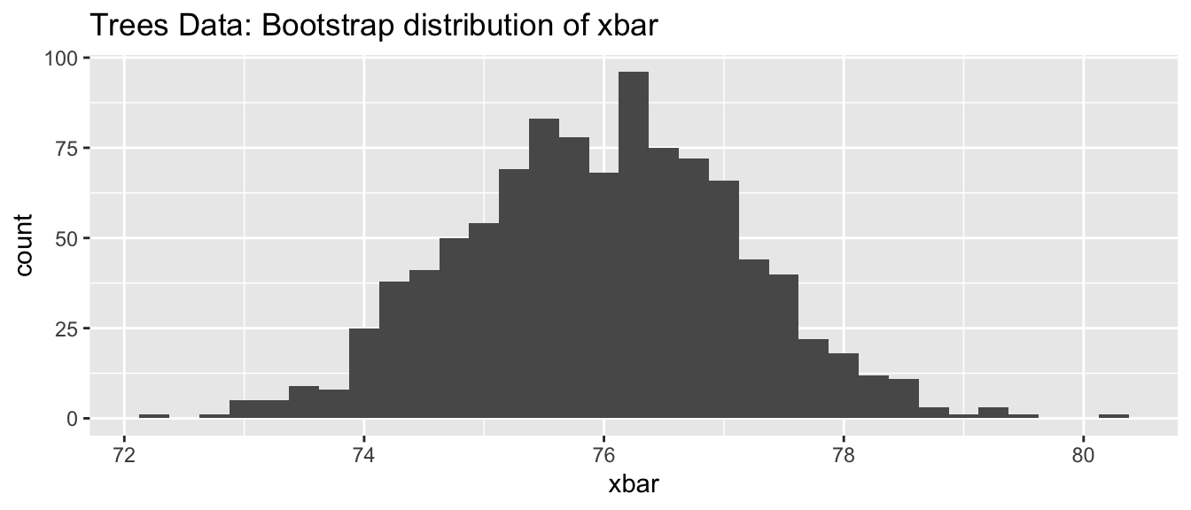

6.3.3 `mosaic::do()` loops

Many times when using a for loop, we want to save some quantity for each pass through the for loop. Because this is such a common tasks, the mosaic::do() function automates the creation of the output data frame and the saving each repetition. This function is intended to hide the coding steps that often trips up new programmers.

# Same Loop 
SampDist <- mosaic::do(1000) * {
  trees %>% dplyr::sample_frac(replace=TRUE)  %>%
    dplyr::summarise(xbar=mean(Height)) %>%       # 1x1 data frame
    pull(xbar)                                    # Scalar 
}

# Structure of the SampDist object 
str(SampDist)

## Classes 'do.data.frame' and 'data.frame':    1000 obs. of  1 variable:
##  $ result: num  77 74.4 74.5 76.6 74 ...
##  - attr(*, "lazy")= language ~{     trees %>% dplyr::sample_frac(replace = TRUE) %>% dplyr::summarise(xbar = mean(Height)) %>%  ...
##   ..- attr(*, ".Environment")=<environment: R_GlobalEnv> 
##  - attr(*, "culler")=function (object, ...)

# Plot the output
ggplot(SampDist, aes(x=result)) + 
  geom_histogram( binwidth=0.25) +
  labs(title='Trees Data: Bootstrap distribution of xbar')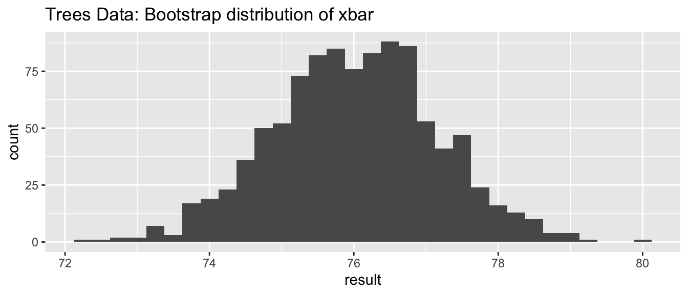

6.4 Functions

It is very important to be able to define a piece of programming logic that is repeated often. For example, I don’t want to have to always program the mathematical code for calculating the sample variance of a vector of data. Instead I just want to call a function that does everything for me and I don’t have to worry about the details.

While hiding the computational details is nice, fundamentally writing functions allows us to think about our problems at a higher layer of abstraction. For example, most scientists just want to run a t-test on their data and get the appropriate p-value out; they want to focus on their problem and not how to calculate what the appropriate degrees of freedom are. Another statistical example where functions are important is a bootstrap data analysis where we need to define a function that calculates whatever statistic the research cares about.

The format for defining your own function is

function.name <- function(arg1, arg2, arg3){
  statement1
  statement2
}

where arg1 is the first argument passed to the function and arg2 is the second.

To illustrate how to define your own function, we will define a variance calculating function.

# define my function
my.var <- function(x){
  n <- length(x)                # calculate sample size
  xbar <- mean(x)               # calculate sample mean
  SSE <- sum( (x-xbar)^2 )      # calculate sum of squared error
  v <- SSE / ( n - 1 )          # "average" squared error
  return(v)                     # result of function is v
}

# create a vector that I wish to calculate the variance of
test.vector <- c(1,2,2,4,5)

# calculate the variance using my function
calculated.var <- my.var( test.vector )
calculated.var

## [1] 2.7

Notice that even though I defined my function using x as my vector of data, and passed my function something named test.vector, R does the appropriate renaming. If my function doesn’t modify its input arguments, then R just passes a pointer to the inputs to avoid copying large amounts of data when you call a function. If your function modifies its input, then R will take the input data, copy it, and then pass that new copy to the function. This means that a function cannot modify its arguments. In Computer Science parlance, R does not allow for procedural side effects. Think of the variable x as a placeholder, with it being replaced by whatever gets passed into the function.

When I call a function, it might cause something to happen (e.g. draw a plot); or, it might do some calculations, the result of which is returned by the function, and we might want to save that. Inside a function, if I want the result of some calculation saved, I return the result as the output of the function. The way I specify to do this is via the return statement. (Actually R doesn’t completely require this. But the alternative method is less intuitive and I strongly recommend using the return() statement for readability.)

By writing a function, I can use the same chunk of code repeatedly. This means that I can do all my tedious calculations inside the function and just call the function whenever I want and happily ignore the details. Consider the function t.test() which we have used to do all the calculations in a t-test. We could write a similar function using the following code:

# define my function
one.sample.t.test <- function(input.data, mu0){
  n    <- length(input.data)
  xbar <- mean(input.data)
  s    <- sd(input.data)
  t    <- (xbar - mu0)/(s / sqrt(n))
  if( t < 0 ){
    p.value <- 2 * pt(t, df=n-1)
  }else{
    p.value <- 2 * (1-pt(t, df=n-1))
  }
  # we haven't addressed how to print things in a organized 
  # fashion, the following is ugly, but works...
  # Notice that this function returns a character string
  # with the necessary information in the string.
  return( paste('t =', round(t, digits=3), ' and p.value =', round(p.value, 3)) )
}

# create a vector that I wish apply a one-sample t-test on.
test.data <- c(1,2,2,4,5,4,3,2,3,2,4,5,6)
one.sample.t.test( test.data, mu0=2 )

## [1] "t = 3.157  and p.value = 0.008"

Nearly every function we use to do data analysis is written in a similar fashion. Somebody decided it would be convenient to have a function that did an ANOVA analysis and they wrote something that is similar to the above function, but is a bit grander in scope. Even if you don’t end up writing any of your own functions, knowing how will help you understand why certain functions you use are designed the way they are.

6.5 Exercises

I’ve created a dataset about presidential candidates for the 2020 US election and it is available on the github website for my STA 141

prez <- readr::read_csv('https://raw.githubusercontent.com/dereksonderegger/444/master/data-raw/Prez_Candidate_Birthdays')
prez

## # A tibble: 11 x 5
##    Candidate        Gender Birthday   Party AgeOnElection
##    <chr>            <chr>  <date>     <chr>         <dbl>
##  1 Pete Buttigieg   M      1982-01-19 D                38
##  2 Andrew Yang      M      1975-01-13 D                45
##  3 Juilan Castro    M      1976-09-16 D                44
##  4 Beto O'Rourke    M      1972-09-26 D                48
##  5 Cory Booker      M      1969-04-27 D                51
##  6 Kamala Harris    F      1964-10-20 D                56
##  7 Amy Klobucher    F      1960-05-25 D                60
##  8 Elizabeth Warren F      1949-06-22 D                71
##  9 Donald Trump     M      1946-06-14 R                74
## 10 Joe Biden        M      1942-11-20 D                77
## 11 Bernie Sanders   M      1941-09-08 D                79

Re-code the Gender column to have Male and Female levels. Similarly convert the party variable to be Democratic or Republican. You may write this using a for() loop with an if(){ ... }else{...} structure nested inside, or simply using a mutate() statement with the ifelse() command inside. I believe the second option is MUCH easier.
Bernie Sanders was registered as an Independent up until his 2016 presidential run. Change his political party value into ‘Independent.’

The \(Uniform\left(a,b\right)\) distribution is defined on x \(\in [a,b]\) and represents a random variable that takes on any value of between a and b with equal probability. Technically since there are an infinite number of values between a and b, each value has a probability of 0 of being selected and I should say each interval of width \(d\) has equal probability. It has the density function \[f\left(x\right)=\begin{cases} \frac{1}{b-a} & \;\;\;\;a\le x\le b\\ 0 & \;\;\;\;\textrm{otherwise} \end{cases}\]

The R function dunif() evaluates this density function for the above defined values of x, a, and b. Somewhere in that function, there is a chunk of code that evaluates the density for arbitrary values of \(x\). Run this code a few times and notice sometimes the result is \(0\) and sometimes it is \(1/(10-4)=0.16666667\).
```
a <- 4      # The min and max values we will use for this example
b <- 10     # Could be anything, but we need to pick something

x <- runif(n=1, 0,10)  # one random value between 0 and 10 

# what is value of f(x) at the randomly selected x value?  
dunif(x, a, b)
```
```
## [1] 0.1666667
```
We will write a sequence of statements that utilizes if statements to appropriately calculate the density of x, assuming that a, b , and x are given to you, but your code won’t know if x is between a and b. That is, your code needs to figure out if it is and give either 1/(b-a) or 0.
1. We could write a set of if else statements.
```
a <- 4
b <- 10
x <- runif(n=1, 0,10)  # one random value between 0 and 10 

if( x < a ){
  result <- ????      # Replace ???? with something appropriate!
}else if( x <= b ){
  result <- ????
}else{
  result <- ????
}
print(paste('x=',round(x,digits=3), '  result=', round(result,digits=3)))
```
  Replace the ???? with the appropriate value, either 0 or \(1/\left(b-a\right)\). Run the code repeatedly until you are certain that it is calculating the correct density value.
2. We could perform the logical comparison all in one comparison. Recall that we can use & to mean “and” and | to mean “or.” In the following two code chunks, replace the ??? with either & or | to make the appropriate result.
  1. ```
  x <- runif(n=1, 0,10)  # one random value between 0 and 10 
  if( (a<=x) ??? (x<=b) ){
    result <- 1/(b-a)
  }else{
    result <- 0
  }
  print(paste('x=',round(x,digits=3), '  result=', round(result,digits=3)))
```
2. ```
x <- runif(n=1, 0,10)  # one random value between 0 and 10 
if( (x<a) ??? (b<x) ){
  result <- 0
}else{
  result <- 1/(b-a)
}
print(paste('x=',round(x,digits=3), '  result=', round(result,digits=3)))
```
  3. ```
  x <- runif(n=1, 0,10)  # one random value between 0 and 10 
  result <- ifelse( a<=x & x<=b, ???, ??? )
  print(paste('x=',round(x,digits=3), '  result=', round(result,digits=3)))
```
I often want to repeat some section of code some number of times. For example, I might want to create a bunch plots that compare the density of a t-distribution with specified degrees of freedom to a standard normal distribution.
```
library(ggplot2)
df <- 5
N <- 1000
x.grid <- seq(-3, 3, length=N)
data <- data.frame( 
  x = c(x.grid, x.grid),
  y = c(dnorm(x.grid), dt(x.grid, df)),
  type = c( rep('Normal',N), rep('T',N) ) )

# make a nice graph
myplot <- ggplot(data, aes(x=x, y=y, color=type, linetype=type)) +
  geom_line() +
  labs(title = paste('Std Normal vs t with', df, 'degrees of freedom'))

# actually print the nice graph we made
print(myplot)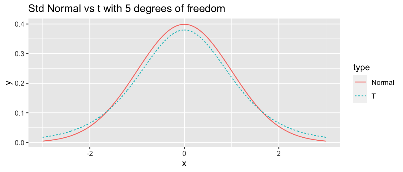 
```
1. Use a for loop to create similar graphs for degrees of freedom \(2,3,4,\dots,29,30\).
2. In retrospect, perhaps we didn’t need to produce all of those. Rewrite your loop so that we only produce graphs for \(\left\{ 2,3,4,5,10,15,20,25,30\right\}\) degrees of freedom. Hint: you can just modify the vector in the for statement to include the desired degrees of freedom.
It is very common to run simulation studies to estimate probabilities that are difficult to work out. In this exercise we will investigate a gambling question that sparked much of the fundamental mathematics behind the study of probability.

The game is to roll a pair of 6-sided dice 24 times. If a “double-sixes” comes up on any of the 24 rolls, the player wins. What is the probability of winning?
1. We can simulate rolling two 6-sided dice using the sample() function with the replace=TRUE option. Read the help file on sample() to see how to sample from the numbers \(1,2,\dots,6\). Sum those two die rolls and save it as throw.
2. Write a for{} loop that wraps your code from part (a) and then tests if any of the throws of dice summed to 12. Read the help files for the functions any() and all(). Your code should look something like the following:
```
throws <- NULL
for( i in 1:24 ){
  throws[i] <- ??????  # Your part (a) code goes here
}
game <- any( throws == 12 ) # Gives a TRUE/FALSE value
```
3. Wrap all of your code from part (b) in another for(){} loop that you run 10,000 times. Save the result of each game in a games vector that will have 10,000 elements that are either TRUE/FALSE depending on the outcome of that game. You’ll need initiallize the games vector to NULL and modify your part (b) code to save the result into some location in the vector games.
4. Finally, calculate win percentage by taking the average of the games vector.

Chapter 6 Flow Control

6.1 Logical Expressions

6.2 Decision statements

6.2.1 In dplyr wrangling

6.2.2 General if else