Chapter 4 Data Wrangling
suppressPackageStartupMessages({
  library(tidyverse, quietly = TRUE)    # loading ggplot2 and dplyr
})
As always, there is a Video Lecture that accompanies this chapter.
Many of the tools to manipulate data frames in R were written without a consistent
syntax and are difficult use together. To remedy this, Hadley Wickham
(the writer of ggplot2) introduced a package called plyr which was quite useful.
As with many projects, his first version was good, but not great, and he introduced
an improved version that works exclusively with data frames called dplyr which
we will investigate. The package dplyr strives to provide a convenient and
consistent set of functions to handle the most common data frame manipulations,
and a mechanism for chaining these operations together to perform complex tasks.
Dr. Wickham has put together a very nice introduction to the package that explains in more detail how the various pieces work and I encourage you to read it at some point. [https://cran.rstudio.com/web/packages/dplyr/vignettes/dplyr.html].
One of the aspects about the data.frame object is that R does some simplification
for you, but it does not do it in a consistent manner. Somewhat obnoxiously,
character strings are always converted to factors and subsetting might return a
data.frame or a vector or a scalar. This is fine at the command line, but
can be problematic when programming. Furthermore, many operations are pretty
slow using data.frame. To get around this, Dr. Wickham introduced a modified
version of the data.frame called a tibble. A tibble is a data.frame but
with a few extra bits. For now we can ignore the differences.
The pipe command %>% allows for very readable code. The idea is that the %>%
operator works by translating the command a %>% f(b) to the expression f(a,b).
This operator works on any function and was introduced in the magrittr package.
This operator is so powerful and useful that it will soon be included as part of
the base functionality of R!
The beauty of the pipe operator comes when you have a suite of functions that
takes input arguments of the same type as their output.
For example, if we wanted to start with x, and first apply function f(),
then g(), and then h(), the usual R command would be h(g(f(x))) which is
hard to read because you have to start reading at the innermost set of
parentheses. Using the pipe command %>%, this sequence of operations
becomes x %>% f() %>% g() %>% h().
| Written | Meaning |
|---|---|
a %>% f(b) |
f(a,b) |
b %>% f(a, .) |
f(a, b) |
x %>% f() %>% g() |
g( f(x) ) |
# This code is not particularly readable because
# the order of summing vs taking absolute value isn't
# completely obvious.
sum(abs(c(-1,0,1)))
## [1] 2# But using the pipe function, it is blatantly obvious
# what order the operations are done in.
c( -1, 0, 1) %>% # take a vector of values
abs() %>% # take the absolute value of each
sum() # add them up.## [1] 2In dplyr, all the functions below take a data set as its first argument
and outputs an appropriately modified data set. This will allow me to chain
together commands in a readable fashion.
For a more precise reasoning why using pipes in your code is superior, consider the following set of function calls that describes my morning routine. In this case, each function takes a person as an input and an appropriately modified person as an output object:
drive(drive(eat_breakfast(shave(clean(get_out_of_bed(wake_up(me), side='right'),
method='shower'), location='face'), what=c('cereal','coffee')),
location="Kid's School"), location='NAU')
The problem with code like this is that the function call parameters are far
away from the function name. So that the function drive() which has a parameter
location='NAU' has the two pieces ridiculously far from each other.
The same set of function calls using a pipe command, keeps the function name and function parameters together in a much more readable format:
me %>%
  wake_up() %>%
  get_out_of_bed(side='right') %>%
  clean( method='shower') %>%
  shave( location='face') %>%
  eat_breakfast( what=c('cereal','coffee')) %>%
  drive( location="Kid's School") %>%
  drive( location='NAU')
By piping the commands together, it is both easier to read, but also easier to modify. Imagine if I am running late and decide to skip the shower and shave. Then all I have to do is comment out those two steps like so:
me %>%
  wake_up() %>%
  get_out_of_bed(side='right') %>%
  # clean( method='shower') %>%
  # shave( location='face') %>%
  eat_breakfast( what=c('cereal','coffee')) %>%
  drive( location="Kid's School") %>%
  drive( location='NAU')
This works so elegantly because the function call and its parameters are together instead of being spread apart and containing all the prior steps. If you wanted to comment out these steps in the first nested statement it is a mess. You end up re-writing the code so that one command is on a single line, but the function call and its parameters are still obnoxiously spread apart and I have to comment out four lines of code and I have to make sure the parameters I comment out are the right ones. Indenting the functions makes that easier, but this is still unpleasant and prone to error.
drive(
  drive(
    eat_breakfast(
      # shave(
      #   clean(
          get_out_of_bed(
            wake_up(me),
          side='right'),
      #   method='shower'),
      # location='face'),
    what=c('cereal','coffee')),
  location="Kid's School"),
location='NAU')
The final way that you might have traditionally written this code without the pipe operator is by saving the output objects of each step:
me2 <- wake_up(me)
me3 <- get_out_of_bed(me2, side='right')
me4 <- clean(me3, method='shower')
me5 <- shave(me4, location='face')
me6 <- eat_breakfast(me5, what=c('cereal','coffee'))
me7 <- drive(me6, location="Kid's School")
me8 <- drive(me7, location='NAU')
But now to remove the clean/shave steps, we have to ALSO remember to
update the eat_breakfast() to use the appropriate me variable.
me2 <- wake_up(me)
me3 <- get_out_of_bed(me2, side='right')
# me4 <- clean(me3, method='shower')
# me5 <- shave(me4, location='face')
me6 <- eat_breakfast(me3, what=c('cereal','coffee'))  # This was also updated!
me7 <- drive(me6, location="Kid's School")
me8 <- drive(me7, location='NAU')
When it comes time to add the clean/shave steps back in, it is far too
easy to forget to update eat_breakfast() command as well
me2 <- wake_up(me)
me3 <- get_out_of_bed(me2, side='right')
me4 <- clean(me3, method='shower')
me5 <- shave(me4, location='face')
me6 <- eat_breakfast(me3, what=c('cereal','coffee'))  # forgot to update this!
me7 <- drive(me6, location="Kid's School")
me8 <- drive(me7, location='NAU')
So to prevent having that problem, programmers will often just overwrite the same object.
me <- wake_up(me)
me <- get_out_of_bed(me, side='right')
me <- clean(me, method='shower')
me <- shave(me, location='face')
me <- eat_breakfast(me, what=c('cereal','coffee'))  # forgot to update this!
me <- drive(me, location="Kid's School")
me <- drive(me, location='NAU')
Aside from still having to write me so often, the original object me has been
overwritten immediately. To write and test the next step in the code chunk,
I have to remember to run whatever code originally produced the me object. That is
really easy to forget to do and this can induce a lot of frustration. So this
results in creating a me_X variable for each code chunk. So we’ll still have
obnoxious numbers of temporary variables. When I add/remove new chunks, I have
to be careful to use the right temporary variables.
With the pipe operator, I typically have a work flow where I keep adding steps and
debugging without overwriting my initial input object. Only once the code-chunk is
completely debugged and I’m perfectly happy with it, will I finally save the
output and overwrite the me object. This simplifies my writing/debugging
process and removes any redundancy in object names.
me <-
  me %>%
  wake_up() %>%
  get_out_of_bed(side='right') %>%
  # clean( method='shower') %>%
  # shave( location='face') %>%
  eat_breakfast( what=c('cereal','coffee')) %>%
  drive( location="Kid's School") %>%
  drive( location='NAU')
So the pipe operator allows us to keep the function call and parameters together and prevents us from having to name/store all the intermediate results. As a result I make fewer programming mistakes and that saves me time and frustration.
4.1 Verbs
The foundational operations to perform on a data set are:
| Adding rows | Adds to a data set |
|---|---|
add_rows() |
Add an additional single row of data, specified by cell. |
bind_rows() |
Add additional row(s) of data, specified by the added data table. |
| Subsetting | Returns a data set with particular columns or rows |
|---|---|
select |
Selecting a subset of columns by name or column number. Helper functions such as starts_with(), ends_with(), and contains() allows you pick columns that have certain attributes in their column names. |
filter() |
Selecting a subset of rows from a data frame based on logical expressions. |
slice() |
Selecting a subset of rows by row number. There are a few variants that allow for common tasks to such as slice_head() slice_tail() and slice_sample() |
drop_na() |
Remove rows that contain any missing values. |
| Sorting | Returns a data table with the rows or columns sorted |
|---|---|
arrange() |
Re-ordering the rows of a data frame. The desc() function can be used on the selected column to reverse the sort direction. |
relocate() |
Moves columns to around. |
| Update/Add columns | Returns a data table updated and/or new column(s). |
|---|---|
mutate() |
Add a new column that is some function of other columns. This function is used with an ifelse() command for updating particular cells and across() to apply some function to a variety of columns. |
| Summarize | Returns a data table with many rows into summarized into one row. |
|---|---|
summarise() |
Calculate some summary statistic of a column of data. This collapses a set of rows into fewer (often one) rows. |
Each of these operations is a function in the package dplyr. These functions
all have a similar calling syntax, the first argument is a data set, subsequent
arguments describe what to do with the input data frame and you can refer to the
columns without using the df$column notation. All of these functions will return
a data set.
To demonstrate all of these actions, we will consider a tiny dataset of a gradebook of doctors at a Sacred Heart Hospital.
# Create a tiny data frame that is easy to see what is happening
Mentors <- tribble(
  ~l.name, ~Gender, ~Exam1, ~Exam2, ~Final,
  'Cox',     'M',     93.2,   98.3,     96.4,
  'Kelso',   'M',     80.7,   82.8,     81.1)
Residents <- tribble(
  ~l.name, ~Gender, ~Exam1, ~Exam2, ~Final,
  'Dorian',  'M',     89.3,   70.2,   85.7,
  'Turk',    'M',     70.9,   85.5,   92.2)
4.1.1 Adding new rows
4.1.1.1 add_row
Suppose that we want to add a row to our dataset. We can give it as much or as
little information as we want and any missing information will be denoted as
missing using a NA which stands for Not Available.
Residents  %>%
  add_row( l.name='Reid', Exam1=95.3, Exam2=92.0)
## # A tibble: 3 x 5
## l.name Gender Exam1 Exam2 Final
## <chr> <chr> <dbl> <dbl> <dbl>
## 1 Dorian M 89.3 70.2 85.7
## 2 Turk M 70.9 85.5 92.2
## 3 Reid <NA> 95.3 92 NABecause we didn’t assign the result of our previous calculation to any object
name, R just printed the result. Instead, lets add all of Dr Reid’s information
and save the result by overwritting the grades data.frame with the new version.
Residents <- Residents %>%
  add_row( l.name='Reid', Gender='F', Exam1=95.3, Exam2=92.0, Final=100.0)
Residents
## # A tibble: 3 x 5
## l.name Gender Exam1 Exam2 Final
## <chr> <chr> <dbl> <dbl> <dbl>
## 1 Dorian M 89.3 70.2 85.7
## 2 Turk M 70.9 85.5 92.2
## 3 Reid F 95.3 92 1004.1.1.2 bind_rows
To combine two data frames together, we’ll bind them together using bind_rows().
We just need to specify the order to stack them.
# now to combine two data frames by stacking Mentors first and then Residents
grades <- Mentors %>%
  bind_rows(Residents)

grades
## # A tibble: 5 x 5
## l.name Gender Exam1 Exam2 Final
## <chr> <chr> <dbl> <dbl> <dbl>
## 1 Cox M 93.2 98.3 96.4
## 2 Kelso M 80.7 82.8 81.1
## 3 Dorian M 89.3 70.2 85.7
## 4 Turk M 70.9 85.5 92.2
## 5 Reid F 95.3 92 1004.1.2 Subsetting
These function allows you select certain columns and rows of a data frame.
4.1.2.1 select()
Often you only want to work with a small number of columns of a data frame and
want to be able to select a subset of columns or perhaps remove a subset.
The function to do that is dplyr::select().
I could select the Exam columns by hand, or by using an extension of the : operator.
# select( grades,  Exam1, Exam2 )   # from `grades`, select columns Exam1, Exam2
grades %>% select( Exam1, Exam2 )   # Exam1 and Exam2
## # A tibble: 5 x 2
## Exam1 Exam2
## <dbl> <dbl>
## 1 93.2 98.3
## 2 80.7 82.8
## 3 89.3 70.2
## 4 70.9 85.5
## 5 95.3 92grades %>% select( Exam1:Final ) # Columns Exam1 through Final## # A tibble: 5 x 3
## Exam1 Exam2 Final
## <dbl> <dbl> <dbl>
## 1 93.2 98.3 96.4
## 2 80.7 82.8 81.1
## 3 89.3 70.2 85.7
## 4 70.9 85.5 92.2
## 5 95.3 92 100grades %>% select( -Exam1 ) # Negative indexing by name drops a column## # A tibble: 5 x 4
## l.name Gender Exam2 Final
## <chr> <chr> <dbl> <dbl>
## 1 Cox M 98.3 96.4
## 2 Kelso M 82.8 81.1
## 3 Dorian M 70.2 85.7
## 4 Turk M 85.5 92.2
## 5 Reid F 92 100grades %>% select( 1:2 ) # Can select column by column position## # A tibble: 5 x 2
## l.name Gender
## <chr> <chr>
## 1 Cox M
## 2 Kelso M
## 3 Dorian M
## 4 Turk M
## 5 Reid FThe select() command has a few other tricks. There are functional calls that
describe the columns you wish to select that take advantage of pattern matching.
I generally can get by with starts_with(), ends_with(), and contains(),
but there is a final operator matches() that takes a regular expression.
grades %>% select( starts_with('Exam') ) # Exam1 and Exam2## # A tibble: 5 x 2
## Exam1 Exam2
## <dbl> <dbl>
## 1 93.2 98.3
## 2 80.7 82.8
## 3 89.3 70.2
## 4 70.9 85.5
## 5 95.3 92grades %>% select( starts_with(c('Exam','F')) ) # All three exams ## # A tibble: 5 x 3
## Exam1 Exam2 Final
## <dbl> <dbl> <dbl>
## 1 93.2 98.3 96.4
## 2 80.7 82.8 81.1
## 3 89.3 70.2 85.7
## 4 70.9 85.5 92.2
## 5 95.3 92 100The select function allows you to include multiple selector helpers.
The help file
for tidyselect package describes a few other interesting selection helper
functions. One final one is the where() command which will apply a function
to each column and return the columns in which the values will evaluate to TRUE.
This is particularly handy for selecting all numeric columns or all columns that
are character strings.
# select only the numerical numerical columns
grades %>% select( where(is.numeric) )
## # A tibble: 5 x 3
## Exam1 Exam2 Final
## <dbl> <dbl> <dbl>
## 1 93.2 98.3 96.4
## 2 80.7 82.8 81.1
## 3 89.3 70.2 85.7
## 4 70.9 85.5 92.2
## 5 95.3 92 100# select numerical or character columns
grades %>% select( where(is.numeric), where(is.character) )The dplyr::select function is quite handy, but there are several other packages
out there that have a select function and we can get into trouble with loading
other packages with the same function names. If I encounter the select function
behaving in a weird manner or complaining about an input argument, my first remedy
is to be explicit about it is the dplyr::select() function by appending the
package name at the start.
4.1.2.2 filter()
It is common to want to select particular rows where we have some logical expression to pick the rows.
# select students with Final grades greater than 90
grades %>% filter(Final > 90)
## # A tibble: 3 x 5
## l.name Gender Exam1 Exam2 Final
## <chr> <chr> <dbl> <dbl> <dbl>
## 1 Cox M 93.2 98.3 96.4
## 2 Turk M 70.9 85.5 92.2
## 3 Reid F 95.3 92 100You can have multiple logical expressions to select rows and they will be logically
combined so that only rows that satisfy all of the conditions are selected. The
logicals are joined together using & (and) operator or the | (or) operator and
you may explicitly use other logicals. For example, a factor column type might be
used to select rows where type is either one or two via the following: type==1 | type==2.
# select students with Final grades above 90 and
# average score also above 90
grades %>% filter(Final > 90, ((Exam1 + Exam2 + Final)/3) > 90)
## # A tibble: 2 x 5
## l.name Gender Exam1 Exam2 Final
## <chr> <chr> <dbl> <dbl> <dbl>
## 1 Cox M 93.2 98.3 96.4
## 2 Reid F 95.3 92 100# we could also use an "and" condition
grades %>% filter(Final > 90 & ((Exam1 + Exam2 + Final)/3) > 90)## # A tibble: 2 x 5
## l.name Gender Exam1 Exam2 Final
## <chr> <chr> <dbl> <dbl> <dbl>
## 1 Cox M 93.2 98.3 96.4
## 2 Reid F 95.3 92 1004.1.2.3 slice()
When you want to filter rows based on row number, this is called slicing.
# grab the first 2 rows
grades %>% slice(1:2)
## # A tibble: 2 x 5
## l.name Gender Exam1 Exam2 Final
## <chr> <chr> <dbl> <dbl> <dbl>
## 1 Cox M 93.2 98.3 96.4
## 2 Kelso M 80.7 82.8 81.1There are a few other slice variants that are useful. slice_head() and
slice_tail grab the first and last few rows. The slice_sample() allows us
to randomly grab table rows.
# sample with replacement, number of rows is 100% of the original number of rows
# This is super helpful for bootstrapping code
grades %>%
  slice_sample(prop=1, replace=TRUE)
## # A tibble: 5 x 5
## l.name Gender Exam1 Exam2 Final
## <chr> <chr> <dbl> <dbl> <dbl>
## 1 Turk M 70.9 85.5 92.2
## 2 Kelso M 80.7 82.8 81.1
## 3 Dorian M 89.3 70.2 85.7
## 4 Cox M 93.2 98.3 96.4
## 5 Cox M 93.2 98.3 96.44.1.3 Sorting via arrange()
We often need to re-order the rows of a data frame. For example, we might wish
to take our grade book and sort the rows by the average score, or perhaps
alphabetically. The arrange() function does exactly that. The first argument
is the data frame to re-order, and the subsequent arguments are the columns to
sort on. The order of the sorting column determines the precedent: the first
sorting column is first used and the second sorting column is only used to break ties.
grades %>% arrange(l.name)## # A tibble: 5 x 5
## l.name Gender Exam1 Exam2 Final
## <chr> <chr> <dbl> <dbl> <dbl>
## 1 Cox M 93.2 98.3 96.4
## 2 Dorian M 89.3 70.2 85.7
## 3 Kelso M 80.7 82.8 81.1
## 4 Reid F 95.3 92 100
## 5 Turk M 70.9 85.5 92.2The default sorting is in ascending order, so to sort the grades with the highest
scoring person in the first row, we must tell arrange to do it in descending order
using desc(column.name).
grades %>% arrange(desc(Final))## # A tibble: 5 x 5
## l.name Gender Exam1 Exam2 Final
## <chr> <chr> <dbl> <dbl> <dbl>
## 1 Reid F 95.3 92 100
## 2 Cox M 93.2 98.3 96.4
## 3 Turk M 70.9 85.5 92.2
## 4 Dorian M 89.3 70.2 85.7
## 5 Kelso M 80.7 82.8 81.1We can also order a data frame by multiple columns.
# Arrange by Gender first, then within each gender, order by Exam2
grades %>% arrange(Gender, desc(Exam2))
## # A tibble: 5 x 5
## l.name Gender Exam1 Exam2 Final
## <chr> <chr> <dbl> <dbl> <dbl>
## 1 Reid F 95.3 92 100
## 2 Cox M 93.2 98.3 96.4
## 3 Turk M 70.9 85.5 92.2
## 4 Kelso M 80.7 82.8 81.1
## 5 Dorian M 89.3 70.2 85.74.1.4 Update and Create new columns with mutate()
The mutate command either creates a new column in the data frame or updates an already existing column.
I often need to create a new column that is some function of the old columns.
In the dplyr package, this is a mutate command. To do this, we give a
mutate( NewColumn = Function of Old Columns ) command. You can do multiple
calculations within the same mutate() command, and you can even refer to columns
that were created in the same mutate() command.
grades <- grades %>%
  mutate(
    average = (Exam1 + Exam2 + Final)/3,
    grade = cut(average, c(0, 60, 70, 80, 90, 100),  # cut takes numeric variable
                         c( 'F','D','C','B','A'))    # and makes a factor
  )

grades
## # A tibble: 5 x 7
## l.name Gender Exam1 Exam2 Final average grade
## <chr> <chr> <dbl> <dbl> <dbl> <dbl> <fct>
## 1 Cox M 93.2 98.3 96.4 96.0 A
## 2 Kelso M 80.7 82.8 81.1 81.5 B
## 3 Dorian M 89.3 70.2 85.7 81.7 B
## 4 Turk M 70.9 85.5 92.2 82.9 B
## 5 Reid F 95.3 92 100 95.8 AIf we want to update some column information we will also use the mutate
command, but we need some mechanism to select the rows to change, while keeping
all the other row values the same. The functions if_else() and case_when()
are ideal for this task.
The if_else syntax is if_else( logical.expression, TrueValue, FalseValue ).
For each row of the table, the logical expression will be evaluated, and if the
expression is TRUE, the TrueValue is selected, otherwise FalseValue is.
We can use this to update a score in our gradebook.
# Update Dr Reid's Final Exam score to 98, and leave everybody else's alone.
grades <- grades %>%
  mutate( Final = if_else(l.name == 'Reid', 98, Final ) )
grades
## # A tibble: 5 x 7
## l.name Gender Exam1 Exam2 Final average grade
## <chr> <chr> <dbl> <dbl> <dbl> <dbl> <fct>
## 1 Cox M 93.2 98.3 96.4 96.0 A
## 2 Kelso M 80.7 82.8 81.1 81.5 B
## 3 Dorian M 89.3 70.2 85.7 81.7 B
## 4 Turk M 70.9 85.5 92.2 82.9 B
## 5 Reid F 95.3 92 98 95.8 AWe could also use this to modify all the rows. For example, perhaps we want to
change the gender column information to have levels Male and Female.
# Update the Gender column labels
grades <- grades %>%
  mutate( Gender = if_else(Gender == 'M', 'Male', 'Female' ) )
grades
## # A tibble: 5 x 7
## l.name Gender Exam1 Exam2 Final average grade
## <chr> <chr> <dbl> <dbl> <dbl> <dbl> <fct>
## 1 Cox Male 93.2 98.3 96.4 96.0 A
## 2 Kelso Male 80.7 82.8 81.1 81.5 B
## 3 Dorian Male 89.3 70.2 85.7 81.7 B
## 4 Turk Male 70.9 85.5 92.2 82.9 B
## 5 Reid Female 95.3 92 98 95.8 ATo do something similar for the case where we have 3 or more categories,
we could use the if_else() command repeatedly to address each category level
separately. However this is annoying to do because the ifelse command is limited
to just two cases, it would be nice if there was a generalization to multiple categories.
The dplyr::case_when function is that generalization.
The syntax is case_when( logicalExpression1~Value1, logicalExpression2~Value2, ... ).
We can have as many LogicalExpression ~ Value pairs as we want.
Consider the following data frame that has name, gender, and political party affiliation of six individuals. In this example, we’ve coded male/female as 1/0 and political party as 1,2,3 for democratic, republican, and independent.
people <- data.frame(
  name = c('Barack','Michelle', 'George', 'Laura', 'Bernie', 'Deborah'),
  gender = c(1,0,1,0,1,0),
  party = c(1,1,2,2,3,3)
)
people
## name gender party
## 1 Barack 1 1
## 2 Michelle 0 1
## 3 George 1 2
## 4 Laura 0 2
## 5 Bernie 1 3
## 6 Deborah 0 3Now we’ll update the gender and party columns to code these columns in a readable fashion.
people <- people %>%
  mutate( gender = if_else( gender == 0, 'Female', 'Male') ) %>%
  mutate( party = case_when( party == 1 ~ 'Democratic',
                             party == 2 ~ 'Republican',
                             party == 3 ~ 'Independent',
                             TRUE       ~ 'None Stated' ) )
people
## name gender party
## 1 Barack Male Democratic
## 2 Michelle Female Democratic
## 3 George Male Republican
## 4 Laura Female Republican
## 5 Bernie Male Independent
## 6 Deborah Female IndependentOften the last case is a catch all case where the logical expression will ALWAYS evaluate to TRUE and this is the value for all other input.
In the above case, we are transforming the variable into a character string.
If we had already transformed party into a factor, we could have used the
command forcats::fct_recode() function instead. See the Factors chapter in this book
for more information about factors.
4.1.4.1 Modify Multiple Columns using across()
We often find that we want to modify multiple columns at once. For example in
the grades, we might want to round the exams so that we don’t have to deal with
any decimal points. To do this, we need to have some code to: 1) select the
desired columns, 2) indicate the function to use, and 3) combine those. The
dplyr::across() function is designed to do this. The across function will
work within a mutate or summarise() function.
grades %>%
  mutate( across(         # Pick any of the following column selection tricks...
    #c('Exam1','Exam2','Final'),        # Specify columns explicitly
    starts_with(c('Exam', 'Final')),    # anything that select can use...
    # where(is.numeric),                # If a column has a specific type..
    # Exam1:Final,                      # Or via a range notation
    round,                # The function I want to use
    digits = 0            # additional arguments sent into round()
  ))
## # A tibble: 5 x 7
## l.name Gender Exam1 Exam2 Final average grade
## <chr> <chr> <dbl> <dbl> <dbl> <dbl> <fct>
## 1 Cox Male 93 98 96 96.0 A
## 2 Kelso Male 81 83 81 81.5 B
## 3 Dorian Male 89 70 86 81.7 B
## 4 Turk Male 71 86 92 82.9 B
## 5 Reid Female 95 92 98 95.8 AIn most of the code examples you’ll find online, this is usually written in a single line of code, which I find somewhat ugly.
grades %>%
  mutate(across(starts_with(c('Exam', 'Final')),  round, digits = 0))
As before, any select helper function will work, and could have rounded
all the numeric columns via the following:
grades %>%
  mutate(across( where(is.numeric), round, digits=0 ))
## # A tibble: 5 x 7
## l.name Gender Exam1 Exam2 Final average grade
## <chr> <chr> <dbl> <dbl> <dbl> <dbl> <fct>
## 1 Cox Male 93 98 96 96 A
## 2 Kelso Male 81 83 81 82 B
## 3 Dorian Male 89 70 86 82 B
## 4 Turk Male 71 86 92 83 B
## 5 Reid Female 95 92 98 96 AIn earlier versions of dplyr there was no across function, but instead there
where variants of mutate and summarise such as mutate_if() that would apply
the desired function to some set of columns. However these made some pretty strong
assumptions about what a user was likely to want to do and, as a result, lacked the
flexibility to handle more complicated scenarios. Those scoped variant functions
have been superseded and users are encouraged to use the across function.
4.1.4.2 Create a new column using many columns
Often we have many many columns in the data frame and we want to utilize all of
them to create a summary statistic. There are several ways to do this, but it
is easiest to utilize the rowwise() and c_across() commands.
The command dplyr::rowwise() causes subsequent actions to be performed
rowwise instead of the default of columnwise. rowwise() is actually a
special form of group_by() which creates a unique group for each row. The
function dplyr::c_across() allows you to use all the select style tricks for
picking columns.
grades %>%
  select(l.name:Final) %>%   # remove the previously calculated average & grade
  rowwise() %>%
  mutate( average = mean( c_across( # Pick any of the following column selection tricks...
    # c('Exam1','Exam2','Final')        # Specify columns explicitly
    starts_with(c('Exam', 'Final'))     # anything that select can use...
    # where(is.numeric)                 # If a column has a specific type..
    # Exam1:Final                       # Or via a range notation
  )) )
## # A tibble: 5 x 6
## # Rowwise:
## l.name Gender Exam1 Exam2 Final average
## <chr> <chr> <dbl> <dbl> <dbl> <dbl>
## 1 Cox Male 93.2 98.3 96.4 96.0
## 2 Kelso Male 80.7 82.8 81.1 81.5
## 3 Dorian Male 89.3 70.2 85.7 81.7
## 4 Turk Male 70.9 85.5 92.2 82.9
## 5 Reid Female 95.3 92 98 95.1Because rowwise() is a special form of grouping, to exit the row-wise
calculations, call ungroup().
4.1.5 summarise()
By itself, this function is quite boring, but will become useful later on. Its purpose is to calculate summary statistics using any or all of the data columns. Notice that we get to chose the name of the new column. The way to think about this is that we are collapsing information stored in multiple rows into a single row of values.
# calculate the mean of exam 1
grades %>% summarise( mean.E1=mean(Exam1) )
## # A tibble: 1 x 1
## mean.E1
## <dbl>
## 1 85.9We could calculate multiple summary statistics if we like.
# calculate the mean and standard deviation
grades %>% summarise( mean.E1=mean(Exam1),
                      stddev.E1=sd(Exam1))
## # A tibble: 1 x 2
## mean.E1 stddev.E1
## <dbl> <dbl>
## 1 85.9 10.14.2 Split, apply, combine
Aside from unifying the syntax behind the common operations, the major strength
of the dplyr package is the ability to split a data frame into a bunch of sub data
frames, apply a sequence of one or more of the operations we just described, and
then combine results back together. We’ll consider data from an experiment from
spinning wool into yarn. This experiment considered two different types of wool
(A or B) and three different levels of tension on the thread. The response variable
is the number of breaks in the resulting yarn. For each of the 6 wool:tension
combinations, there are 9 replicated observations.
data(warpbreaks)
str(warpbreaks)
## 'data.frame': 54 obs. of 3 variables:
## $ breaks : num 26 30 54 25 70 52 51 26 67 18 ...
## $ wool : Factor w/ 2 levels "A","B": 1 1 1 1 1 1 1 1 1 1 ...
## $ tension: Factor w/ 3 levels "L","M","H": 1 1 1 1 1 1 1 1 1 2 ...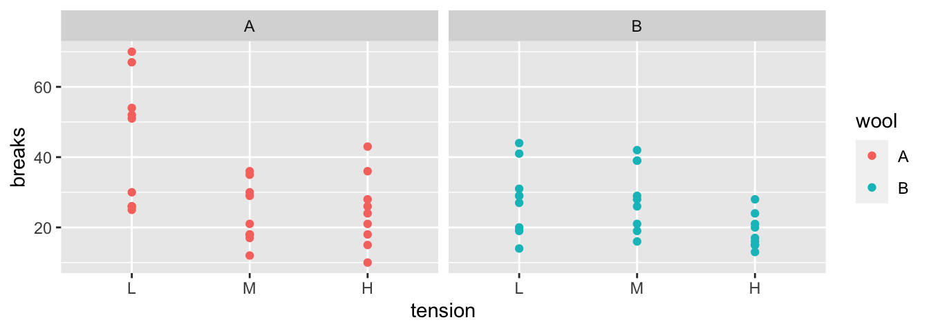
The first we must do is to create a data frame with additional information about how to break the data into sub data frames. In this case, I want to break the data up into the 6 wool-by-tension combinations. Initially we will just figure out how many rows are in each wool-by-tension combination.
# group_by:  what variable(s) shall we group on.
# n() is a function that returns how many rows are in the
#   currently selected sub dataframe
# .groups tells R to drop the grouping structure after doing the summarize step
warpbreaks %>%
  group_by( wool, tension) %>%                   # grouping
  summarise(n = n(), .groups='drop')             # how many in each group
## # A tibble: 6 x 3
## wool tension n
## <fct> <fct> <int>
## 1 A L 9
## 2 A M 9
## 3 A H 9
## 4 B L 9
## 5 B M 9
## 6 B H 9The group_by function takes a data.frame and returns the same data.frame, but
with some extra information so that any subsequent function acts on each unique
combination defined in the group_by. If you wish to remove this behavior, use
group_by() or ungroup() to reset the grouping to have no grouping variable.
The summarise() function collapses many rows into fewer rows. a single row and therefore
it is natural to update the grouping structure during the call tosummarise.
The options are to drop grouping completely, drop_last to drop the last level
of grouping, keep the same grouping structure, or turn every row into its own
group with rowwise.
For several years dplyr did not require the .groups option because summarise
only allowed for single row results. In version 1.0.0, a change was made to allow
summarise to only collapse the group to fewer rows and that means the choice
of resulting grouping should be thought about. While the default behavior to
drop_last if all the results have 1 row makes sense, the user really should
specify what the resulting grouping should be.
Using the same summarise function, we could calculate the group mean and
standard deviation for each wool-by-tension group.
summary_table <-
  warpbreaks %>%
  group_by(wool, tension) %>%
  summarize( n           = n() ,             # I added some formatting to show the
             mean.breaks = mean(breaks),     # reader I am calculating several
             sd.breaks   = sd(breaks),       # statistics.
             .groups = 'drop')               # drop all grouping structure
If instead of summarizing each split, we might want to just do some calculation
and the output should have the same number of rows as the input data frame. In
this case I’ll tell dplyr that we are mutating the data frame instead of
summarizing it. For example, suppose that I want to calculate the residual
value \[e_{ijk}=y_{ijk}-\bar{y}_{ij\cdot}\] where \(\bar{y}_{ij\cdot}\) is the mean
of each wool:tension combination.
warpbreaks %>%
   group_by(wool, tension) %>%                 # group by wool:tension
   mutate(resid = breaks - mean(breaks)) %>%   # mean(breaks) of the group!
   head(  )                                    # show the first couple of rows
## # A tibble: 6 x 4
## # Groups: wool, tension [1]
## breaks wool tension resid
## <dbl> <fct> <fct> <dbl>
## 1 26 A L -18.6
## 2 30 A L -14.6
## 3 54 A L 9.44
## 4 25 A L -19.6
## 5 70 A L 25.4
## 6 52 A L 7.444.3 Exercises
The dataset
ChickWeighttracks the weights of 48 baby chickens (chicks) feed four different diets. Feel free to complete all parts of the exercise in a single R pipeline at the end of the problem.Load the dataset using
data(ChickWeight)Look at the help files for the description of the columns.
- Remove all the observations except for observations from day 10 or day 20.
The tough part in this instruction is distinguishing between “and” and “or.”
Obviously there are no observations that occur from both day 10 AND day 20.
Google ‘R logical operators’ to get an introduction to those, but the
short answer is that and is
&and or is|. - Calculate the mean and standard deviation of the chick weights for each diet group on days 10 and 20.
The OpenIntro textbook on statistics includes a data set on body dimensions. Instead of creating an R chunk for each step of this problem, create a single R pipeline that performs each of the following tasks.
Load the file using
Body <- read.csv('http://www.openintro.org/stat/data/bdims.csv')The column
sexis coded as a 1 if the individual is male and 0 if female. This is a non-intuitive labeling system. Create a new columnsex.MFthat uses labels Male and Female. Use this column for the rest of the problem. Hint: Theifelse()command will be very convenient here. It functions similarly to the same command in Excel.The columns
wgtandhgtmeasure weight and height in kilograms and centimeters (respectively). Use these to calculate the Body Mass Index (BMI) for each individual where \[BMI=\frac{Weight\,(kg)}{\left[Height\,(m)\right]^{2}}\]Double check that your calculated BMI column is correct by examining the summary statistics of the column (e.g.
summary(Body)). BMI values should be between 18 to 40 or so. Did you make an error in your calculation?
The function
cuttakes a vector of continuous numerical data and creates a factor based on your given cut-points.# Define a continuous vector to convert to a factor x <- 1:10 # divide range of x into three groups of equal length cut(x, breaks=3)## [1] (0.991,4] (0.991,4] (0.991,4] (0.991,4] (4,7] (4,7] (4,7] ## [8] (7,10] (7,10] (7,10] ## Levels: (0.991,4] (4,7] (7,10]# divide x into four groups, where I specify all 5 break points cut(x, breaks = c(0, 2.5, 5.0, 7.5, 10))## [1] (0,2.5] (0,2.5] (2.5,5] (2.5,5] (2.5,5] (5,7.5] (5,7.5] (7.5,10] ## [9] (7.5,10] (7.5,10] ## Levels: (0,2.5] (2.5,5] (5,7.5] (7.5,10]# (0,2.5] (2.5,5] means 2.5 is included in first group # right=FALSE changes this to make 2.5 included in the second # divide x into 3 groups, but give them a nicer # set of group names cut(x, breaks=3, labels=c('Low','Medium','High'))## [1] Low Low Low Low Medium Medium Medium High High High ## Levels: Low Medium HighCreate a new column of in the data frame that divides the age into decades (10-19, 20-29, 30-39, etc). Notice the oldest person in the study is 67.
Body <- Body %>%
  mutate( Age.Grp = cut(age,
                        breaks=c(10,20,30,40,50,60,70),
                        right=FALSE))
Find the average BMI for each
Sex.MFbyAge.Grpcombination.
Suppose we have a data frame with the following two variables:
df <- tribble(
  ~SubjectID, ~Outcome,
  1, 'good',
  1, 'good',
  1, 'good',
  2, 'good',
  2, 'bad',
  2, 'good',
  3, 'bad',
  4, 'good',
  4, 'good')
The
SubjectIDrepresents a particular individual that has had multiple measurements. What we want to know is what proportion of individuals were consistentlygoodfor all outcomes they had observed. So in our toy example set, subjects1and4where consistently good, so our answer should be \(50\%\). Hint: The steps below help understand the thinking, but this problem can be done in two lines of code.- As a first step, we will summarize each subject with a column
denotes if all the subject’s observations were
good. This should result in a column of TRUE/FALSE values with one row for each subject. Theall()function should be quite useful here. The correspondingany()function is also useful to know about. - Calculate the proportion of subjects that where consistently good by
calculating the
mean()of the TRUE/FALSE values. This works because TRUE/FALSE values are converted to 1/0 values and then averaged.
- As a first step, we will summarize each subject with a column
denotes if all the subject’s observations were