Chapter 17 Data Scraping
suppressPackageStartupMessages({
  library(tidyverse)
  library(rvest)     # rvest is not loaded in the tidyverse Metapackage
})
I have a YouTube Video Lecture for this chapter, as usual.
Getting data into R often involves accessing data that is available through non-convenient formats such as web pages or .pdf files. Fortunately those formats still have structure and we can import data from those sources. However to do this, we have to understand a little bit about those file formats.
17.1 Web Pages
Posting information on the web is incredibly common. As we first use google to find answers to our problems, it is inevitable that we’ll want to grab at least some of that information and import it as data into R. There are several ways to go about this:
Human Copy/Paste - Sometimes it is easy to copy/paste the information into a spreadsheet. This works for small datasets, but sometimes the HTML markup attributes get passed along and this suddenly becomes very cumbersome for more than a small amount of data. Furthermore, if the data is updated, we would have to redo all of the work instead of just re-running or tweaking a script.
Download the page, parse the HTML, and select the information you want. The difficulty here is knowing what you want in the raw HTML tags.
Knowing how web pages are generated is certainly extremely helpful in this endeavor, but isn’t absolutely necessary. It is sufficient to know that HTML has open and closing tags for things like tables and lists.
# Example of HTML code that would generate a table
# Table Rows    begin and end with <tr> and </tr>
# Table Data    begin and end with <td> and </td>
# Table Headers begin and end with <th> and </th>
<table style="width:100%">
  <tr> <th>Firstname</th> <th>Lastname</th>     <th>Age</th>  </tr>
  <tr> <td>Derek</td>     <td>Sonderegger</td>  <td>43</td>   </tr>
  <tr> <td>Aubrey</td>    <td>Sonderegger</td>  <td>39</td>   </tr>
</table>
# Example of an unordered List, which starts and ends with <ul> and </ul>
# Each list item is enclosed by <li> </li>
<ul>
<li>Coffee</li>
<li>Tea</li>
<li>Milk</li>
</ul>Given this extremely clear structure it shouldn’t be too hard to grab tables and/or lists from a web page. However HTML has a heirarchical structure so that tables could be nested in lists. In order to control the way the page looks, there is often a lot of nesting. For example, we might be in a split pane page that has a side bar, and then a block that centers everything, and then some style blocks that control fonts and colors. Add to this, the need for modern web pages to display well on both mobile devices as well as desktops and the raw HTML typically is extremely complicated. In summary the workflow for scraping a web page will be:
- Find the webpage you want to pull information from.
- Download the html file
- Parse it for tables or lists (this step could get ugly!)
- Convert the HTML text or table into R data objects.
Hadley Wickham wrote a package to address the need for web scraping functionality and it happily works with the usual magrittr pipes. The package rvest is intended to harvest data from the web and make working with html pages relatively simple.
17.1.1 Example Wikipedia Table
Recently I needed to get information about U.S. state population sizes. I did a quick googling and found a Wikipedia page that has the information that I wanted.
url = 'https://en.wikipedia.org/wiki/List_of_states_and_territories_of_the_United_States_by_population'

# Download the web page and save it. I like to do this within a single R Chunk
# so that I don't keep downloading a page repeatedly while I am fine tuning
# the subsequent data wrangling steps.
page <- read_html(url)
# Once the page is downloaded, we need to figure out which table to work with.
# There are 5 tables on the page.
page %>%
html_nodes('table') ## {xml_nodeset (5)}
## [1] <table class="wikitable sortable" style="width:100%; text-align:center;"> ...
## [2] <table class="wikitable"><tbody>\n<tr><th style="text-align: left;">Legen ...
## [3] <table class="wikitable sortable" style="text-align: right;">\n<caption>P ...
## [4] <table class="nowraplinks hlist mw-collapsible autocollapse navbox-inner" ...
## [5] <table class="nowraplinks hlist mw-collapsible mw-collapsed navbox-inner" ...With five tables on the page, I need to go through each table individually and decide if it is the one that I want. To do this, we’ll take each table and convert it into a data.frame and view it to see what information it contains.
# This chunk of code is a gigantic pain. Because Wikipedia can be edited by anybody,
# There are a couple of people that keep changing this table back and forth, sometimes
# with different numbers of columns, sometimes with the columns moved around.  This
# is generally annoying because everytime I re-create the notes, this section of code
# breaks. This is a great example of why you don't want to scrap data in scripts that
# have a long lifespan.
State_Pop <-
  page %>%
  html_nodes('table') %>%
  .[[1]] %>%                              # Grab the first table and
  html_table(header=FALSE, fill=TRUE) %>% # convert it from HTML into a data.frame
  # magrittr::set_colnames(c('Rank_current','Rank_2010','State',
  #           'Population2020', 'Population2010',
  #           'Percent_Change','Absolute_Change',                            #
  #           'House_Seats', 'Population_Per_Electoral_Vote', #)) %>%        #
  #           'Population_Per_House_Seat', 'Population_Per_House_Seat_2010', # Wikipedia keeps changing these
  #           'Percent_US_Population')) %>%                                  # columns.  Aaarggh!
  slice(-1 * 1:2 )

# Just grab the three columns that seem to change the least frequently.  Sheesh!
State_Pop <- State_Pop %>%
  select(3:5) %>%
  magrittr::set_colnames( c('State', 'Population2020','Population2010') )

# To view this table, we could use View() or print out just the first few
# rows and columns. Converting it to a tibble makes the printing turn out nice.
State_Pop %>% as_tibble()
## # A tibble: 60 x 3
## State Population2020 Population2010
## <chr> <chr> <chr>
## 1 California 39,368,078 37,253,956
## 2 Texas 29,360,759 25,145,561
## 3 Florida 21,733,312 18,801,310
## 4 New York 19,336,776 19,378,102
## 5 Pennsylvania 12,783,254 12,702,379
## 6 Illinois 12,587,530 12,830,632
## 7 Ohio 11,693,217 11,536,504
## 8 Georgia 10,710,017 9,687,653
## 9 North Carolina 10,600,823 9,535,483
## 10 Michigan 9,966,555 9,883,640
## # … with 50 more rowsIt turns out that the first table on the page is the one that I want. Now we need to just do a little bit of clean up by renaming columns, and turning the population values from character strings into numbers. To do that, we’ll have to get rid of all those commas. Also, the rows for the U.S. territories have text that was part of the footnotes. So there are [7], [8], [9], and [10] values in the character strings. We need to remove those as well.
State_Pop <- State_Pop %>%
  select(State, Population2020, Population2010) %>%
  mutate_at( vars(matches('Pop')), str_remove_all, ',') %>%           # remove all commas
  mutate_at( vars(matches('Pop')), str_remove, '\\[[0-9]+\\]') %>%    # remove [7] stuff
  mutate_at( vars( matches('Pop')), as.numeric)                       # convert to numbers
And just to show off the data we’ve just imported from Wikipedia, we’ll make a nice graph.
State_Pop %>%
  filter( !(State %in% c('Contiguous United States',
                        'The fifty states','Fifty states + D.C.',
                        'Total U.S. (including D.C. and territories)') ) )  %>%
  mutate( Percent_Change = (Population2020 - Population2010)/Population2010 ) %>%
  mutate( State = fct_reorder(State, Percent_Change) ) %>%
ggplot( aes(x=State, y=Percent_Change) ) +
  geom_col( ) +
  labs(x=NULL, y='% Change', title='State Population growth 2010-2020') +
  coord_flip() +
theme(text = element_text(size = 9)) 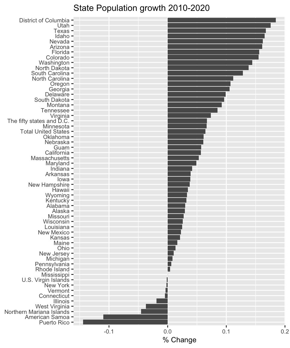
17.1.2 Lists
Unfortunately, we don’t always want to get information from a webpage that is nicely organized into a table. Suppose we want to gather the most recent threads on Digg.
We could sift through the HTML tags to find something that will match, but that will be challenging. Instead we will use a CSS selector named SelectorGadget. Install the bookmarklet by dragging the following javascript code SelectorGadge up to your browser’s bookmark bar. When you are at the site you are interested in, just click on the SelectorGadget javascript bookmarklet to engage the CSS engine. Click on something you want to capture. This will highlight a whole bunch of things that match the HTML tag listed at the bottom of the screen. Select or deselect items by clicking on them and the search string used to refine the selection will be updated. Once you are happy with the items being selected, copy the HTML node selector. Things highlighted in green are things you clicked on to select, stuff in yellow is content selected by the current html tags, and things in red are things you chose to NOT select.
url <- 'http://digg.com'
page <- read_html(url)
# Once the page is downloaded, we use the SelectorGadget Parse string
# To just give the headlines, we'll use html_text()
HeadLines <- page %>%
html_nodes('.headline a') %>% # Grab just the headlines
html_text() # Convert the <a>Text</a> to just Text
HeadLines %>%
head()## character(0)# Each headline is also a link. I might want to harvest those as well
Links <- page %>%
html_nodes('.headline a') %>%
html_attr('href')
Links %>%
head()## character(0)17.2 Exercises
At the Insurance Institute for Highway Safety, they have data about human fatalities in vehicle crashes. From this web page, import the data from the Fatal Crash Totals data table and produce a bar graph gives the number of deaths per 100,000 individuals. Be sure to sort the states by highest to lowest mortality. Hint: If you have a problem with the graph being too squished vertically, you can set the chunk options
fig.heightorfig.widthto make the graph larger, but keeping the font sizes the same. The result is that the text is more spread apart. The chunk optionsout.heightandout.widthshrink or expand everything in the plot. By making thefix.XXXoptions large andout.XXXoptions small, you are effectively decreasing the font size of all the elements in the graph. The other trick is to reset the font size using a themeelement_textoption:theme(text = element_text(size = 9)).From the same IIHS website, import the data about seat belt use. Join the Fatality data with the seat belt use and make a scatter plot of percent seat belt use vs number of fatalities per 100,000 people.
From the NAU sub-reddit, extract the most recent threads.