4 Estimation vs. testing
The two major approaches to statistical inference are the testing and estimation approaches. This module covers the historical development of popular approaches to both, how the approaches are connected, some critiques of both, and some advice on using them in practice.
4.1 The testing approach to inference
The testing approach uses data to test a single hypothesis, or to choose between competing hypotheses. There are frequentist and Bayesian approaches to testing.
What we call “hypothesis testing” or sometimes “null hypothesis significance testing” (aka NHST) can be traced back to two different approaches, both introduced in the first half of the \(20^{th}\) century.
4.1.1 Fisher’s Significance Testing
“Significance testing” was originally put forth by Ronald Fisher as a method for assessing how much a set of data agree or disagree with a hypothesis, using a p-value.
The p-value is interpreted as quantifying how strongly the data disagree with the hypothesis being tested.
This hypothesis could be a standard “null” hypothesis of today, representing the absence of a theorized “true” effect. But, it doesn’t have to be this kind of hypothesis. One could set up a hypothesis that represents a prediction made by a theory, and test whether data disagree with this prediction.
Fisher’s approach does not involve an “alternative” hypothesis. There is only the null, or what Fisher called the “test hypothesis”.
Fisher recommended the 5% level of significance for testing, but was not strict about it. Some relevant quotes:
“If P is between .1 and .9 there is certainly no reason to suspect the hypothesis tested. If it is below .02 it is strongly indicated that the hypothesis fails to account for the whole of the facts. We shall not often be astray if we draw a conventional line at .05…”
“It is usual and convenient for experimenters to take 5 per cent as a standard level of significance, in the sense that they are prepared to ignore all results which fail to reach this standard, and, by this means, to eliminate from further discussion the greater part of the fluctuations which chance causes have introduced into their experimental results.” (Side note: this is a piece of advice that can produce nasty side effects; see section 5.3.1 for the details.)
“We thereby admit that no isolated experiment, however significant in itself, can suffix for the experimental demonstration of any natural phenomenon … In order to assert that a natural phenomenon is experimentally demonstrable we need, not an isolated record, but a reliable method of procedure. In relation to the test of significance, we may say that a phenomenon is experimentally demonstrable when we know how to conduct an experiment which will rarely fail to give us a statistically significant result”
4.1.2 Neyman and Pearson’s Hypothesis Testing
Neyman and Pearson introducted “hypothesis testing”, which differed from Fisher’s “significance testing” in some important ways:
An alternative hypothesis was introduced, usually denoted as \(H_A\) or \(H_1\). The purpose of the test is to choose between \(H_0\) and \(H_1\); in this sense it hypothesis testing is a decision making procedure.
The two possible decisions were “reject \(H_0\)” and “accept \(H_0\)”. These days the language “accept \(H_0\)” is discouraged; under the original hypothesis testing framework this language was not so objectionable, for reasons we’ll see in a moment.
Type I and Type II error rates must be declared. A Type I error is rejecting a true \(H_0\). A Type II error is accepting a false \(H_0\).
Neyman and Pearson considered hypothesis testing to be tool for decision making, not a method that tells you what to believe. In their words:
“We are inclined to think that as far as a particular hypothesis is concerned, no test based upon a theory of probability can by itself provide any valuable evidence of the truth or falsehood of a hypothesis”
Since the goal was decision making, these was no particular need for using the p-value method; comparing a test statistic to a critical value is mathematically equivalent to comparing a p-value to \(\alpha\). P-values are valuable for Fisher because they have a meaningful probabilistic interpretation, but Neyman and Pearson’s hypothesis testing procedure prioritizes making a choice between \(H_0\) and \(H_1\), not intepreting the statistic used to make that choice.
The strength of an inference made from a hypothesis test was given by its error rates. The researcher states the Type I and Type II error rates, then states the decision. The decision is justified on the grounds of these error rates, e.g. “I am accepting \(H_0\) using a procedure that has a Type II error rate of 10%”.
Power analysis was introduced, as statistical power is defined as the probability of committing a Type II error (i.e, the test leads to rejecting the null hypothesis when the null hypothesis is false), and the declaring a Type II error rate is an important component of hypothesis testing.
Neyman and Pearson’s approach for choosing a test statistic was to first state a Type I error rate, and then choose a test statistic that makes the Type II error rate as small as possible, subject to the Type I error rate. This means that the best test is the test that gives the most statistical power, given the Type I error rate selected.
A few notes on hypothesis testing:
The language “accept \(H_0\)” is discouraged today because it sounds like “the data suggest that \(H_0\) is true” or “we should believe that \(H_0\) is true”. The original purpose of hypothesis testing was strictly decision making. One makes a decision, and states the error rate for the method used to make the decision. Choosing to act as though \(H_0\) is true is not to be confused with choosing to believe that \(H_0\) is true.
As with significance testing, there is no rule that the null hypothesis needs to represent “there is no effect.” Neyman and Pearson envisioned their method as being used to test against competing substantive scientific hypotheses, e.g. by identifying predictions made by the two scientific hypotheses, and using statistical hypothesis testing to choose between them. The modern null of “no effect” is sometimes called the “nil hypothesis” or “nil null”.
4.1.3 One sided vs. two sided tests
Some popular parameters can show the “direction” of an effect via sign. For instance, \(\mu_1-\mu_2\) is negative if \(\mu_2>\mu_1\) and positive if \(\mu_1>\mu_2\). A “two-sided” alternative allows \(H_0\) to be rejected for both negative and positive effects. A “one-sided” alternative states a single direction, and \(H_0\) is only rejected when the parameter’s direction is in line with the alternative (e.g. \(\bar{x}_1>\bar{x}_2\) cannot reject \(H_0\) if \(H_A\) says \(\mu_1-\mu_2<0\)).
The plots below show rejection cutoffs for right-sided and two-sided t-tests testing against \(H_0:\mu_1-\mu_2=0\) (degrees of freedom are 50, but this is not important).
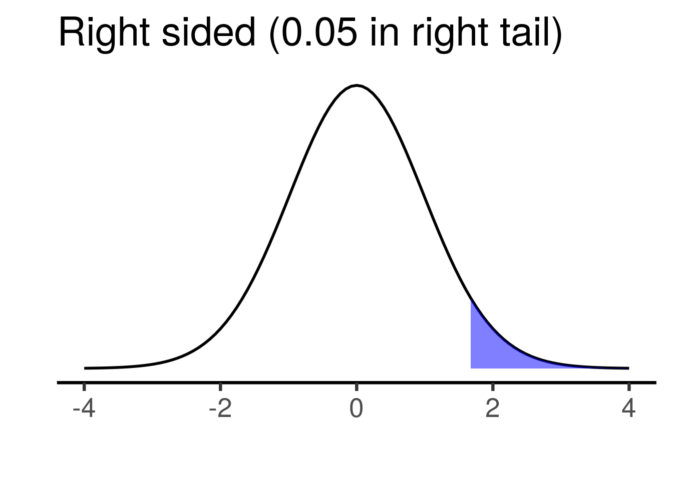
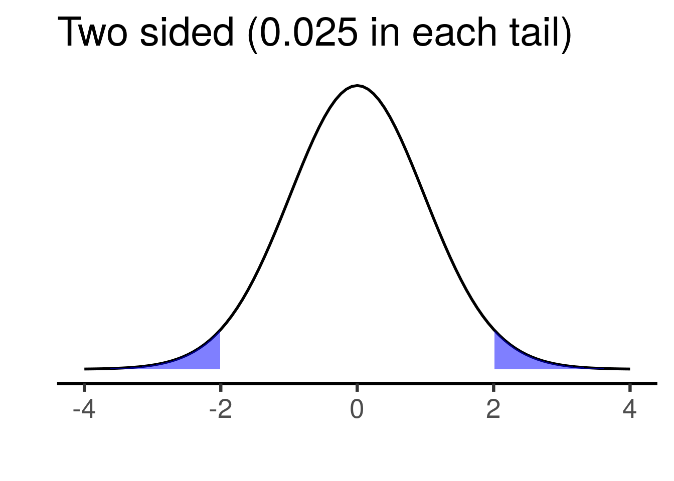
For the right-sided test, the shaded region on the right is \(\alpha=0.05\), and \(H_0\) is rejected in favor of \(H_A: \mu_1-\mu_2>0\) if the test statistic is greater than the corresponding “critical” value (in this case, \(t=1.68\)). For the two-sided test, each shaded region is \(\alpha /2 =0.025\), and \(H_0\) is rejected in favor of \(H_A: \mu_1-\mu_2 \neq0\) if the test statistic is below the left or above the right critical values (in this case, \(t=\pm 2.01\)).
Note that, in either case, the Type 1 error rate is \(\alpha=0.05\). This means that, if the null hypothesis is true, we have a 5% chance of rejecting it. For the right-sided test, a Type I error occurs if the null is true and we get a test statistic above the 95th percentile value of t. For the two-sided test, a Type I error occurs if the null is true and we get a test statistic either below the 2.5 percentile or above the 97.5 percentile.
4.1.3.1 How to write the hypotheses for a one-sided test
Suppose we are doing a right-sided, two-sample t-test, where \(H_A: \mu_1-\mu_2>0\). How should we write the null hypothesis? There are two reasonable options:
A: \(H_0: \mu_1-\mu_2\leq0\) (the “composite” null) B: \(H_0: \mu_1-\mu_2=0\) (the “point” null)
The case for \(H_0: \mu_1-\mu_2\leq0\) is that, when combined with \(H_A\), it covers all possible values of \(\mu_1-\mu_2\). If the alternative is “\(\mu_1\) is bigger than \(\mu_2\)”, this null says “no it isn’t”.
The case for \(H_0: \mu_1-\mu_2=0\) is that we only actually test against the null value of zero. We can say that, if we reject zero, we’d also reject any null value below zero. But the calculation is performed against the null of zero and that is all. Also, since we aren’t supposed to “accept” the null hypothesis, it doesn’t matter if it doesn’t cover all values not in the alternative.
4.1.3.2 Cheating with a one-sided test
What about if we look at our data first, see the sign of the difference in means (negative or positive), and choose to do a one-sided test in the direction of the difference we’ve already observed? If we did this, we’d increase our actual Type I error rate to 10%, because our test statistic could never fall on the side of the distribution opposite the critical value. We can verify this with simulation:
set.seed(335)
reps <- 1e4
N <- 12
pvals <- rep(0,reps)
for (i in 1:reps) {
  sample1 <- rnorm(n=N)
  sample2 <- rnorm(n=N)
  if (mean(sample1)>mean(sample2)) {
    pvals[i] <- t.test(sample1,sample2,alternative="greater")$p.value
  } else {
    pvals[i] <- t.test(sample1,sample2,alternative="less")$p.value
  }
}
sum(pvals<0.05)/reps
## [1] 0.0991Remember that the p-value’s interpretation is a thought experiment about what would happen if the null were true and you performed the same analysis on new data. If you are prepared to adjust your analysis after looking at your data, this thought experiment is a poor reflection of your actual method of analysis.
So, should we be skeptical of one-sided tests? Is it best to default to using two-sided tests? There are arguments for and against both.
4.1.3.3 The case for two-sided tests
As we just saw, one-sided tests can be gamed. If the test statistic’s sign agrees with the direction of the test (right-sided for positive test statistics; left-sided for negative ones), then the critical value is smaller and so it is easier to reject \(H_0\). The one-sided test’s p-value will be half the size of the corresponding two-sided test’s p-value. If the direction of the test is set prior to seeing any data, this is not a concern; under the null there’s a 50% chance the test statistic will fall on the opposite side from the critical value, in which case \(H_0\) cannot be rejected and the p-value will be very large (larger than 0.5). But what if we doubt this? The two-sided test cannot be gamed in this manner, so a skeptic might insist on doubling a one-sided test’s p-value in order to turn it into a two-sided p-value.
A one-sided test can only reject \(H_0\) in one direction, whereas a two-sided test can reject in either direction. What if you’re testing an intervention that is supposed to have a positive effect, but in actuality it is counterproductive?17 If you are performing a one-sided test in the expected direction, your test is not capable of declaring significance in the unexpected direction. So, if there’s a chance you may be wrong about direction and you want to be able to “detect” this, you should use a two-sided test.
If you don’t have a prior expectation about which mean should be bigger than the other if \(H_0\) is true, you should definitely use a two-sided test.
4.1.3.4 The case for one-sided tests
Most real-world hypotheses are directional. For example, pharmaceutical researchers are aren’t going to develop and bring to trial a blood pressure drug with no real-world hypothesis about whether it should make blood pressure go up or go down. If the real-world hypothesis is directional, shouldn’t the statistical hypothesis match it?
While it’s true that people can “cheat” with one-sided tests, there are plenty of other ways for people to cheat in hypothesis testing. If we are going to accept hypothesis testing we are obligated to assume good faith on the part of the researcher.
Two-sided tests (usually) require a “point null”, meaning that the null hypothesis is a single value and the alternative is all other values on either side of it. Do we believe that such a point null could actually be true? “The effect is exactly zero” seems far less plausible than “the effect is in the opposite direction of what I expected”.
If the point null isn’t true, then the result of every two-sided test is either a correct rejection or a Type II error. This is of particular concern when sample sizes are large, making the power to reject a false \(H_0\) larger. In this sense it can be too easy to reject a two-sided null, since you don’t have to pick a direction before collecting data.
My own opinion: I have a philosophical preference for one-sided tests over two-sided tests, because I think they are a better reflection of most real-world hypotheses. But I must also admit that I get a little skeptical when I see a one-sided p-value of 0.035, because I know that the two-sided p-value would be 0.07. If a one-sided test is used, it should be obvious to the reader how its direction was chosen.
4.1.4 Bayesian approaches
There are Bayesian hypothesis testing approaches, in which priors are incorporated and combined with data in order to choose between competing statistical hypotheses.
A popular method uses a “Bayes factor”, which compares the probability of data under two competing hypotheses. Prior probabilities of the two hypotheses are incorporated via Bayes’ Rule. If we call our hypotheses \(H_0\) and \(H_A\),
\[ \frac{P(data|H_A)}{P(data|H_0)}=\frac{\frac{P(H_A|data)P(data)}{P(H_A)}}{\frac{P(H_0|data)P(data)}{P(H_0)}}=\frac{P(H_A|data)P(H_0)}{P(H_0|data)P(H_A)} \]
Some notes:
The Bayes factor quantifies how much the data changes the posterior probability of each hypothesis relative to its prior probability, then gives the ratio of the two. It can be interpreted as how much the data changes the relative probability of \(H_A\) to \(H_0\).
- If the prior probabilities are equal, the Bayes factor tells you how much more likely the numerator hypothesis is than the denominator hypothesis, after incorporating the data.
- If the prior probabilities are not equal, the Bayes factor adjusts the above ratio by giving relatively more weight to the posterior probability of the hypothesis that started with a smaller prior probability.
Example: suppose the posterior probabilities of \(H_0\) and \(H_A\) are both 0.4, but their prior probabilities were 0.75 and 0.25 respectively. Then we have a Bayes factor of \(\frac{0.4\cdot 0.75}{0.4\cdot 0.25}\) = 3, telling us that the ratio of \(P(H_A)\) to \(P(H_0)\) is 3 times greater after observing the data than it was before observing the data.
\(H_0\) and \(H_A\) can refer to single hypothesized parameter values (e.g. \(H_0:\mu=10\) vs \(H_A:\mu=15\)) or ranges of values (e.g. \(H_0:\mu<0\) vs \(H_A:\mu>0\)) or a combination of both. A single hypothesized value will have a prior probability; a range of values will have a prior distribution across these values.
4.1.5 Evidence vs. decisions
In frequentist testing, the p-value is a popular statistic that quantifies how much the data “disagree” with a null hypothesis. Smaller values are thought of as showing stronger evidence against the null.
In Bayesian testing, the Bayes factor is a popular statistic that quantifies how much the data change the probability of one hypothesis compared to another. This is thought of as showing how much evidence the data provide for one hypothesis compared to the other.
In either case, there is no requirement that a “decision” be made. One can report a p-value without saying “therefore I reject \(H_0\)” or “therefore I do not reject \(H_0\)”. One can report a Bayes factor without saying “therefore I chose hypothesis A over hypothesis B”.
We are using the phrase “statistical test” here to refer to methods that use data to quantify evidence for or against a hypothesis. This does not necessarily have to be followed by a formal decision. Some people have a strong preference for stating a decision; some have a strong aversion to it.
4.1.6 Statistical hypotheses vs. scientific hypotheses
Statistical hypotheses are usually set up so that they’ll reflect a “real world” scientific hypothesis. A statistical model is stated, followed by a null hypothesis under that model. An example: We are testing the scientific hypothesis that text message reminders make it more likely that registered voters will choose to vote. Let \(Y\) be a Bernoulli distributed binary variable indicating whether a registered voter chose to vote in the last election. The Bernoulli distribution is a one-parameter probability distribution for modeling binary data. The one parameter is the probability that \(Y=1\), and is denoted \(\pi\).
We run an experiment where known registered voters are randomly assigned to receive or not receive text message reminders, and then we look at updated voter rolls to see if each person voted. Here is the model and null hypothesis, where \(i=1\) for those receiving a reminder and \(i=2\) otherwise, and \(j=1...n_i\) represents the different individual registered voters in each group:
$Y_{1j}\sim Bernoulli(\pi_1)$

$Y_{2j}\sim Bernoulli(\pi_2)$

$H_0:\pi_1 - \pi_2 = 0$
This model seems to represent the scientific hypothesis well, but it is not the scientific hypothesis itself. Some differences:
We assume there is a single “population” probability of voting for those getting reminders, and another population probability for those who don’t. In reality, the probability that someone votes is influenced by far more than just receipt or non-receipt of a reminder. This model is ignorant of any other factors, and effectively treats them as all perfectly averaging out between the two groups.
The model treats the effect of the reminder as additive. This doesn’t seem realistic when we imagine different possible starting probabilities. If the initial probability of voting is 0.6 and a reminder increases this to 0.7, then \(\pi_1-\pi_2=0.1\). What if the initial probability is 0.06? Do we think a reminder would increase this to 0.16?
“All registered voters” isn’t really the “population” of interest, because lots of people either always vote or never vote. The purpose of the text reminder is to increase the probability of voting for people who sometimes vote. This is a harder population to define and to sample from, but the model is ignorant of this distinction.
The idea that there is a population of voters who receive the reminder and a population who do not is itself a thought experiment. Even if our real-world population is well defined, the parameters in this model only make sense as hypothetical statements: if every single registered voter received a text reminder to vote, what proportion would vote? One could argue that the scientific hypothesis makes this thought experiment as well, but it doesn’t have to: it could be interpreted as describing only the voting behavior of actual people get the reminder vs. actual people who do not, with no appeal to a “population”.
We will consider the differences between statistical models and the real world again in module 8.
4.1.7 Testing against scientific hypotheses vs. testing against statistical hypotheses
There is a popular approach to scientific hypothesis testing known as falsificationism. Under the falsificationist approach, hypotheses are tested through the use of experiments that would be capable of falsifying the hypothesis, were the hypothesis false (the idea that hypotheses can be strictly “true” or that they can be shown definitively false is controversial, in which case we might say that our experiment should be capable of showing the ways in which a hypothesis might be deficient or flawed).
This approach was popularized by the philosopher Karl Popper. Popper’s argument is that it is extremely difficult (maybe impossibe) to show definitively that a hypothesis is true, because it could always be false in a manner you are simply unaware of. But, it is simple to show a hypothesis to be false: you just need to show that a logical consequence of the hypothesis does not hold true.
The falsificationist approach has been integrated from philosophy into statistics most notably by philosopher Deborah Mayo, who advocates for a “severe testing” approach to statistical inference.
In brief, a scientific hypothesis is subjected to a critical or severe test, meaning a test that would be highly likely to show the hypothesis to be false if it is indeed false. If the hypothesis fails the test, it is rejected. If it survives the test, we just say that it has survived our attempt to falsify it; we don’t claim to have shown it to be true.
This looks a lot like statistical null hypothesis significance testing (NHST). Under NHST, \(H_0\) is subjected to potential rejection using an approach that has some statistical power (hopefully high) to reject it, if is false. But if \(H_0\) is not rejected, we don’t claim to have shown it to be true.
There is, however, a very important difference between the scientific and statistical approaches to hypothesis testing described above. Under the statistical NHST approach, the null is set to up to represent the scientific hypothesis being false (e.g. “the difference in population mean outcomes for the experimental groups is zero”). And so, the scientific hypothesis is not what is being subjected to potential rejection Rather, what is subjected to potential rejection is the scientific hypothesis being wrong in some particular manner.
Statistical NHST thus appears to be a confirmationist approach to hypothesis testing, rather than a falsificationist approach. The scientific test, according to the falsificationist approach, is capable of falsifying the scientific hypothesis, but cannot show it to be true. Whereas the null hypothesis test is capable of falsifying a particular version of “not the scientific hypothesis”, but cannot show “not the scientific hypothesis” to be true.
This point is explored more deeply in one of the assigned articles for this class:
[meehl_1967_theorytesting]
Important: this is a criticism of NHST as popularly practiced, but NHST is only one version of statistical hypothesis testing. There is no requirement that statistical tests be directed against a “null” hypothesis set up to represent the absence of a real world effect. A statistical test can be directed against a consequence of a scientific hypothesis being true, rather than false. It can be set up to test two scientific hypotheses against each other, rather than one scientific hypothesis against “nothing”.
4.2 The estimation approach to inference
So far, we have looked at three testing approaches to inference:
Fisher’s significance testing, in which a p-value is used to quantify the extent to which data contradict a test hypothesis, and a “significant” deviation from the test hypothesis is declared if the p-value falls below some conventional threshold (usually 0.05).
Neyman and Pearson’s hypothesis testing, in which data are used to make a choice between two competing hypotheses (typically called “null” and “alternative”), and that choice is justified by appealing to the Type I and Type II error rates of the testing procedure.
Bayes factors, which quantify the extent to which data give support to one hypothesis over the other. This is achieved by comparing the ratio of prior probabilities for the two hypotheses to the ratio of posterior probabilities of the two hypotheses; the change from prior to posterior represents the effect of the data on the probability of that hypothesis being true.
The first and third of these produce statistics that are meant to be interpreted. The second is strictly a decision making procedure. What they all have in common is that they require hypotheses.
The estimation approach differs fundamentally from the testing approach in that it does not require hypotheses. Rather, it requires an unknown quantity of interest, and the goal is to use data to draw inference on this unknown quantity.
4.2.1 Point estimates and confidence intervals
Suppose there is some unknown quantity \(\theta\), which is taken to exist at the population level. \(\theta\) could represent all kinds of quantities. Examples:
- The effectiveness of a medical intervention, defined as average outcome for those receiving the intervention minus average outcome for those not receiving the intervention, at the population level.
- The population level correlation between money spent on advertisements aired on podcasts and subsequent change in revenue (for US based companies).
- The proportion of all registered US voters who intend to vote in the next mid-tern election.
We collect data, and we calculate the kind of value that \(\theta\) represents. This is a point estimate for theta. Examples:
The proportion of registered voters in a survey who intend to vote in the next mid-term election is a “point estimate” for the proportion of all registered voters who intend to vote in the mid-term election.
The difference in mean outcomes between participants in a control group and those in an intervention group is a “point estimate” for the difference between:
- Mean outcome for all people in the population, were they to be assigned to the control group
- Mean outcome for all people in the population, were they to be assigned to the intervention group.
If an estimator is unbiased, then its “expected value” is the population level quantity being estimated. But, we don’t actually expect that the numeric value of any one particular statistical estimate will be equal to the value of the population parameter that it estimates18.
Confidence Intervals: A confidence interval is created using a method that, under some assumptions, would achieve the desired “success rate” over the long run, if we were to keep taking new samples and keep calculating new confidence intervals. A “success” is defined as the unknown population-level value being contained within a confidence interval.
Confidence intervals have some good selling points relative to hypothesis testing and p-values:
The parameter being estimated is usually constructed to represent a real-world quantity of interest, and so the confidence interval’s interpretation should be of obvious real-world interest.
They convey magnitude using the units of the original outcome variable (e.g. dollars, velocity, age, etc), rather than in units of probability that seems to confuse people.
They convey the precision of an estimate via their width (if two different confidence intervals have different widths but are estimating the same unknown parameter, the wider one suggests a less precise estimate).
4.2.2 Confidence intervals as inverted hypothesis tests
Jerzy Neyman, who developed hypothesis testing, also developed confidence intervals. The basic connection between the two is this: find all the possible vales for the test (aka null) hypothesis that would not be rejected if tested against using the data at hand. The confidence interval contains all of these values.
This approach should make sense; we are “confident” that the true population parameter value is one that our data does not reject. We would be suspicious of proposed parameter values that our data would reject.
It turns out that intervals made in this matter also achieve their desired coverage rate. Make intervals that contain all values that your data would not reject at the \(\alpha=0.05\) level, and 95% of the time these intervals will contain the unknown parameter value.
4.2.3 Bayesian credible intervals
Bayesians create intervals to represent uncertainty, too. They call theirs “credible intervals”. The interpretation of a credible interval is one that is not allowed for confidence intervals. If you have a 95% credible interval for \(\theta\), you can say that there is a 95% chance the unknown parameter is in that interval.
Example: if we have a 95% credible interval for \(\beta_1\) of \((1.47,5.88)\), then there is a 95% chance that \(\beta_1\) lies somewhere between 1.47 and 5.88.
4.2.4 Confidence intervals as conveying more information than p-values or statistical significance
There is a strong case to be made that confidence intervals are objectively more informative than p-values or statements regarding significance. The argument is that, given a confidence interval, one can calculate the corresponding p-value for a desired null hypothesis. But the converse isn’t true: given a p-value for some null hypothesis, there are an infinity of possible confidence intervals that would produce that p-value.
Visual example:
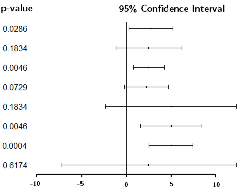
Notice:
As expected, the intervals containing zero produce \(p>0.05\), and those not containing zero produce \(p<0.05\).
There are some confidence intervals that are different, but have the same p-value. This is possible because the point estimate and width of the interval are both changing.
There are some confidence intervals with nearly identical point estimates and similar widths, but that lead to opposite decisions about whether to reject the null hypothesis. And so we should resist the urge to treat results that disagree in terms of significance as though they also disagree in terms of effect size estimate.
Any confidence interval containing zero also contains non-zero values that also wouldn’t be rejected. Thus it is incoherent to say “the parameter is probably zero” just because zero is in the interval: why not pick some other point?
A case for reporting confidence intervals rather than p-values is this: given that a confidence interval can be used to conduct a hypothesis test, it is not clear what is to be gained from reporting a p-value as well. But, if only a p-value had been reported, also reporting a confidence interval would give the reader an estimate for the quantity of interest, surrounded by bounds that represent uncertainty in that estimate. (Exception: some hypothesis tests do not have a corresponding interpretable statistic on which inference can be drawn by inverting the test)
4.3 First applied example: heart stent study
https://www.nytimes.com/2017/11/02/health/heart-disease-stents.html
This New York Times article describes a randomized controlled trial (RCT) to assess the effectiveness of heart stents on easing chest pain.
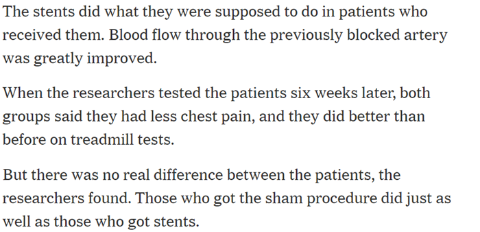
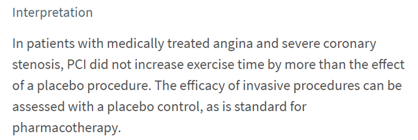
The article claims that the stents were shown not to work. Here is the original paper describing the study and the results:
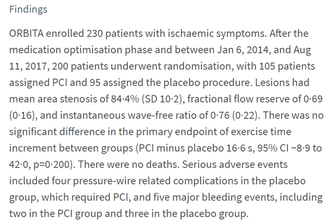
We see here that the primary outcome of interest was amount of time (in seconds) patients were able to spend exercising on a treadmill. The 95% CI for the mean difference between treatment and placebo groups is \((-8.9,42)\), which contains zero.
In the paper, this is interpreted as, essentially, “the null is true”:
Remember, the 95% CI was (-8.9, 42). Zero seconds is a “plausible” value for the difference; so is 33 seconds. So is any value in that confidence interval. (If the researchers had stated ahead of time that they would not be interested in any average improvement less than, say, 60 seconds, this 95% CI could be interpreted as showing that any effect of heart stents on chest pain is too small.)
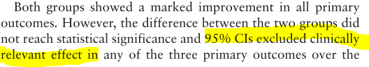
4.4 Second applied example: knee surgery
 Here is another study on the effectiveness of a surgical procedure. Link here
This one is about knee surgery. As with the previous example, this as a randomized controlled trial (RCT) in which roughly half the participants underwent a placebo surgery. And, it is another study in which no “significant” evidence was found to support the effectiveness of the real procedure relative to placebo.
We will look at a 2-year follow up study, performed by the same researchers:

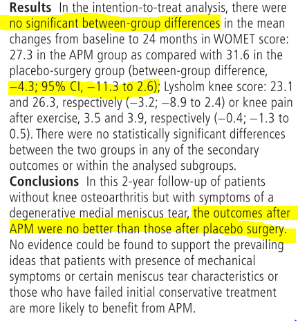
The 95% CI for the difference in mean outcomes between “real” and “sham” surgery groups was \((-11.3,2.6)\), with negative values indicating improvement on an index score (“WOMET”) quantifying severity of symptoms and disability.
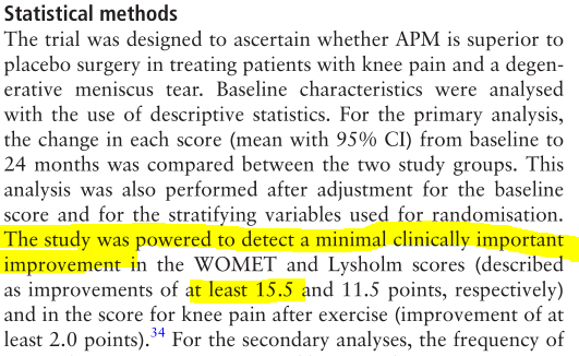
Here, we see that the researchers identified the minimum “clinically important improvement” in WOMET score to be 15.5.
4.5 Critiques of testing
We’ll briefly outline the major critiques of the testing approach, some of which have already come up. These are arguments that you may or may not find convincing, and that are sometimes topics of debate among statisticians and philosophers.
4.5.1 Implausible nulls
The Meehl and Tukey papers on Canvas both argue that a “point” null hypothesis of zero is usually implausible. This is a major challenge to standard null hypothesis significance testing (NHST): if the null was implausible before data were collected, what do we learn when we say that the data lead us to reject this null?
4.5.2 Unnecessary dichotomization
Suppose we have calculated a p-value of 0.018. We declare the result “statistically significant”, because \(p<0.05\).
What was the purpose of the second sentence above? The reader can see that the p-value is 0.018. What additional information is conveyed by pointing out that 0.018 is smaller than 0.05? Since it is obvious to anyone that 0.018 < 0.05, the only reason for pointing this out must be that there is something special about 0.05. Is there?
The story is the same for p-values greater than 0.05. Suppose we get a p-value of 0.088. We would only expect to get a test statistic at least as large as ours 8.8% of the time, if the null were true. This, according to the “p < 0.05” standard, is not good enough. Does the act of declaring 0.088 “not good enough” convey more information than would have been conveyed by simply reporting 0.088?
The Neyman-Pearson hypothesis testing approach says that this is a decision making procedure, and so a cutoff is required. The practical question, then, is: what is being decided? If the decision is simply between saying “reject \(H_0\)” and “do not reject \(H_0\)”, then the decision is trivial: we are using a decision making procedure because we want to decide between two phrases. What is the purpose of this? If the choice between “reject” and “do not reject” is meant to inform our belief regarding the truth of the null, then the problem of prior belief comes into play. It seems like the dichotomous decision procedure is only justified if there is an actionable decision to be made.
4.5.3 Tiny significant effects
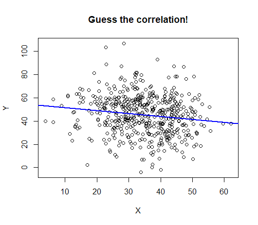
An estimated effect can be very small and also “statistically significant”. Here is an example:
 The data displayed have a highly statistically significant correlation: \(p = 0.0008\)
The correlation itself is -0.15:
 This happens often when sample sizes are large. Here is a study that used ebay data and compared male and female buyers and sellers:

From the results:
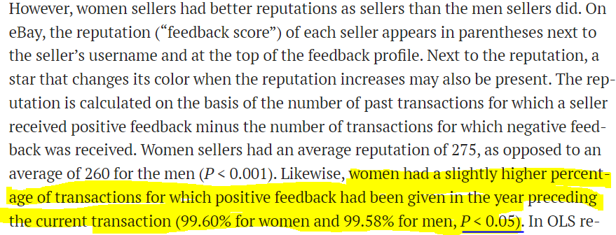
This was a serious study that came to non-trivial conclusions. It is hard to imagine the authors would have bothered to report a difference in probability of 0.0002 (or 0.02 percentage points), had it not been accompanied by “p < 0.05”.
4.5.4 “Not significant” \(\neq\) “not real”
This has been covered in previous notes many times, so we won’t belabor it here. Failure to reject a null hypothesis cannot be taken as evidence that the null hypothesis is true. If we are taking a Bayesian approach and assigning a prior probability to \(H_0\), then it is true that failing to reject \(H_0\) will make the posterior probaility of \(H_0\) increase by some amount relative to the prior. It is also true that, if a study is very highly powered to detect some specified effect, then a failure to reject \(H_0\) is suggestive that the effect is at least smaller than the one the study was powered to. But, it is a fallacy to presume that failing to reject \(H_0\) implies that the null is probably true.
4.6 In support of testing
4.6.1 Testing hypotheses is integral to science
A common retort to critiques of testing is that, for science to progress, we must test hypotheses. It is fine to report estimates, but for a science that cares about theory and explanation, claims must be made and tested against. Otherwise we have a pile of numbers and no way to decide between competing explanations or competing theories.
4.6.2 Sometimes the null hypothesis really is plausible
The critique that “the null is implausible” (made by Tukey and Meehl) only holds when the null is… implausible. If the null is plausible prior to seeing any data, then rejecting it coveys real information. Some examples…
4.6.2.1 “The Lady Tasting Tea”
Perhaps the most famous example of hypothesis testing was given by Fisher in his book “The Design of Experiments”:
“A lady declares that by tasting a cup of tea made with milk she can discriminate whether the milk or the tea infusion was first added to the cup. We will consider the problem of designing an experiment by means of which this assertion can be tested. [It] consists in mixing eight cups of tea, four in one way and four in the other, and presenting them to the subject for judgment in a random order. The subject has been told in advance of that the test will consist, namely, that she will be asked to taste eight cups, that these shall be four of each kind”
(Side note: the “lady” was a scientist and colleague of Fisher’s, Dr. Muriel Bristol, who studied algae. She preferred the milk be poured in first.)
Here, the null hypothesis is that she cannot tell from taste whether the tea or the milk was poured in first. (The implied alternative is that she can tell, but remember that Fisher did not state explicit alternatives!) The p-value will be the probability of correctly identifying at least as many cups as she correctly identifies, assuming this null is true (i.e. by pure guessing).
Notice that this null is EXTREMELY PLAUSIBLE!!!, and so we might be interested if it turns out our data contradict it. If you think she’s just randomly guessing, you’d be surprised by a small p-value.
4.6.2.2 Quality control
In statistical applications to quality control in manufacturing, a typical null hypothesis will be along the lines of “this machine is working properly”.
A distribution of some measured outcome is found (often by simply observing outcomes when the machine is working properly). If an outcome occurs that is very unlikely under this distribution, it’s a good idea to have a technician inspect the machine for problems.
Again, notice that this null is not only EXTREMELY PLAUSIBLE, but also:
- The nullshould in fact be the typical state of things.
- Actual “repeated sampling” is occurring (as opposed to being a thought experiment)
- The sampling distribution of our outcome under the null is observed, rather than being dervied under a set of assumptions
- A cutoff for rejecting the null needs to be used so that we know when to bring over a technician.
4.6.2.3 Extreme case (an XKCD cartoon)
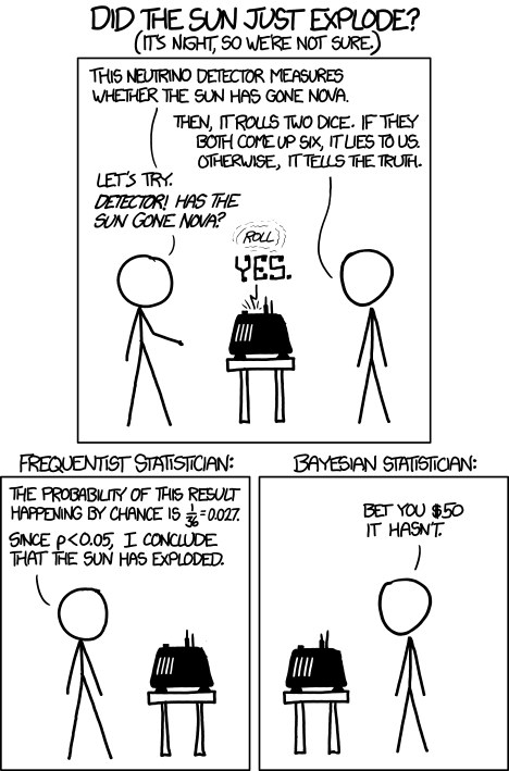
No competent statistician would come to this “conclusion”, at least in the sense that “conclude” implies “believe”. The mistake here is, of course, failing to take into account that…
The null is EXTREMELY PLAUSIBLE!!!In this case, the null is so mind-blowingly overwhelmingly plausible that it seems silly to even bother testing against it.
Lesson: before deciding whether to look at a p-value, ask yourself: do I believe that this null could potentially be true in the first place? Would a p-value give me interesting information?
(Side note: a Bayesian might retort that if we’re going to consider the “plausibility” of a null hypothesis, we should quit being coy and assign it a prior probability)
4.6.3 We don’t want to be fooled by randomness
The original motivation for significance testing was that it is very easy to see patterns in random or noisy data. Just as a cloud might look like a face, raw data might look like a trend. Significance testing is a tool for determining if we think it’s reasonable to conclude that there is a “signal” in noisy data.
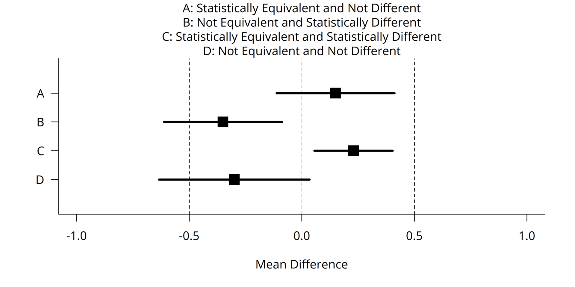
4.7 One compromise: testing interval nulls
We saw a sign of compromise in the knee surgery example: not only was the surgey “not significantly different” from placebo, but the largest value in its 95% confidence interval was smaller than the minimum level of improvement that would be considered valuable.
Stating a “smallest effect size of interest” (SESOI) allows for a null hypothesis that is neither a point value (e.g. \(H_0: \beta_1 = 0\)), nor an inequality that goes out to inifnity (e.g. \(H_0: \beta_1<0\)). Rather, the null is an interval.
- To reject such a null, a confidence interval must be entirely above the SESOI.
- Such a null can be “accepted” if a confidence interval lies entirely below the SESOI, as we saw in the knee surgery example.
- Formal method: “Equivalence testing”: