2 Classical inference
In statistics, “classical” nearly always means “frequentist”.6 Classical (frequentist) statistical inferences are justified on the basis of the long run relative frequency properties of the methods used.7
For example, the “confidence” we have in a confidence interval is justified by the long run success rate of the method, where “success” means capturing whatever quantity the confidence interval is designed to capture, and “long run” implies taking new samples of data from the same population over and over again. This is usually referred to as “repeated sampling”. So…
A 95% confidence interval for a population mean \(\mu\) is made using a method that, under repeated sampling, should capture \(\mu\) 95% of the time.
An 80% confidence interval for a regression coefficent \(\beta_1\) is made using a method that, under repeated sampling, should capture \(\beta_1\) 80% of the time.
Hypothesis testing is also justified on the basis of long run relative frequency. Suppose we perform a hypothesis test at \(\alpha=0.05\) and we reject the null hypothesis. The strength of our inference that the null is false is based upon the fact that our test has a 5% Type I error rate. This means that, if the null hypothesis was true and we were to repeatedly sample from the sample population, we would expect only 5% of these samples to result in mistakenly rejecting this true null.8
This module will go through the details of classical inference, showing how we arrive at the long run relative frequencies that justify our procedures.
2.1 Data as a random sample from a population
Say you collect some data and conduct a statistical analysis. In reporting the results of your analysis, you include a standard error, a confidence interval, and a p-value.
These statistics all have common interpretations that rest upon assumptions. Two such assumptions are that your sample was collected at random from a larger population, and that it is one of many samples that could have been taken from that population.\(^*\)
Let’s simulate this (we’re going to use simulation a lot in DSCI 335).
\(^*\) Do not take these assumptions too literally. We will consider the role of assumptions in chapter 8; for now it is enough to think of them as “thought experiments”: suppose that our sample is one of many that could have been taken from some larger population.
Suppose we are taking a random sample of turnips grown on a plot of land, and measuring their bulb diameter (we plan to compare bulb diameter for turnips grown using different kinds of fertilizers)9.
We treat our sample as having come from a larger population. This population is often hypothetical. In this example, we’ve grown turnips a certain way using a certain fertilizer. So, our population might be “all turnips grown in the exact same conditions as these, were they to receive this fertilizer.”
We will assume that the population of bulb diameters from which ours came is normally distributed with mean diameter of 4.3cm and standard deviation of 0.92cm: \(Diameter\sim Normal(\mu=4.3,\sigma=0.92)\)
The following code simulates taking a single sample from this population of size n = 13. Note: set.seed(335) is included to make sure we get the same results each time we run this simulation. Choose a different seed number, get different results.
set.seed(335)
turnip_sample <- rnorm(n=13,mean=4.3,sd=0.92)
turnip_sample
## [1] 3.382881 3.848617 2.704747 3.862421 5.178445 3.396326 3.723022 3.564967
## [9] 3.973951 3.522526 3.300502 1.627019 3.445757Ok, those are the bulb diameters from our sample. Now we can summarize our sample.
mean(turnip_sample)## [1] 3.502399sd(turnip_sample)## [1] 0.79355592.2 Constructing a sampling distribution
Classical inference always involves appealing to what would happen if we kept taking new samples. So, let’s take a new sample from the same “population”:
turnip_sample_2 <- rnorm(n=13,mean=4.3,sd=0.92)
turnip_sample_2
## [1] 3.334214 4.812136 3.065635 3.169166 3.894195 4.645360 2.511214 4.020288
## [9] 2.935717 5.526864 4.129535 4.791813 3.386930mean(turnip_sample_2)## [1] 3.863313sd(turnip_sample_2)## [1] 0.8921635Not surprisingly, the mean and standard deviation from this sample aren’t the same as from the last one, but they are similar.
Let’s do this a few more times, then look at all the means and standard deviations. (The c() function in R is for “combine”. Here we’re just making a vector of means and a vector of standard deviations)
turnip_sample_3 <- rnorm(n=13,mean=4.3,sd=0.92)
turnip_sample_4 <- rnorm(n=13,mean=4.3,sd=0.92)
turnip_sample_5 <- rnorm(n=13,mean=4.3,sd=0.92)
turnip_means <- c(mean(turnip_sample),mean(turnip_sample_2),mean(turnip_sample_3),mean(turnip_sample_4),mean(turnip_sample_5))
turnip_std_devs <- c(sd(turnip_sample),sd(turnip_sample_2),sd(turnip_sample_3),sd(turnip_sample_4),sd(turnip_sample_5))
cbind(turnip_means,turnip_std_devs)
## turnip_means turnip_std_devs
## [1,] 3.502399 0.7935559
## [2,] 3.863313 0.8921635
## [3,] 4.390105 0.7803646
## [4,] 4.541237 1.0259722
## [5,] 3.964327 1.0087332We now have 5 “samples” of turnip bulb diameters, all taken from the same population. For each sample we have the mean and the standard deviation. We can plot them…
hist(turnip_means,col="grey",
     main="Five means from five samples",
     xlab="Sample means from 5 samples (n=13 each) of bulb diameter")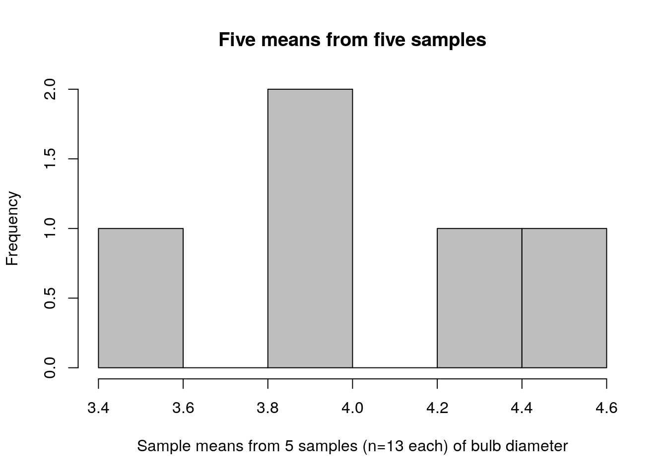
hist(turnip_std_devs,col="grey",
     main="Five standard deviations from five samples",
     xlab="Sample standard deviations from 5 samples (n=13 each) of bulb diameter")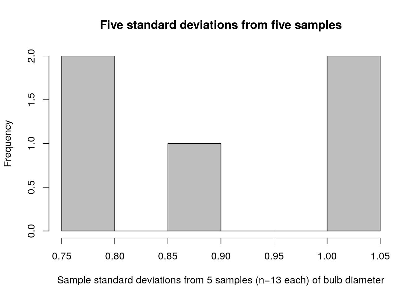
Take a look again at the means and standard deviations; notice that these are the values plotted above:
cbind(turnip_means,turnip_std_devs)## turnip_means turnip_std_devs
## [1,] 3.502399 0.7935559
## [2,] 3.863313 0.8921635
## [3,] 4.390105 0.7803646
## [4,] 4.541237 1.0259722
## [5,] 3.964327 1.0087332Extremely important: the plots above are NOT plots of data! A plot of data looks like this:
hist(turnip_sample_3,main="",col="grey",xlab = "bulb diameter (cm)")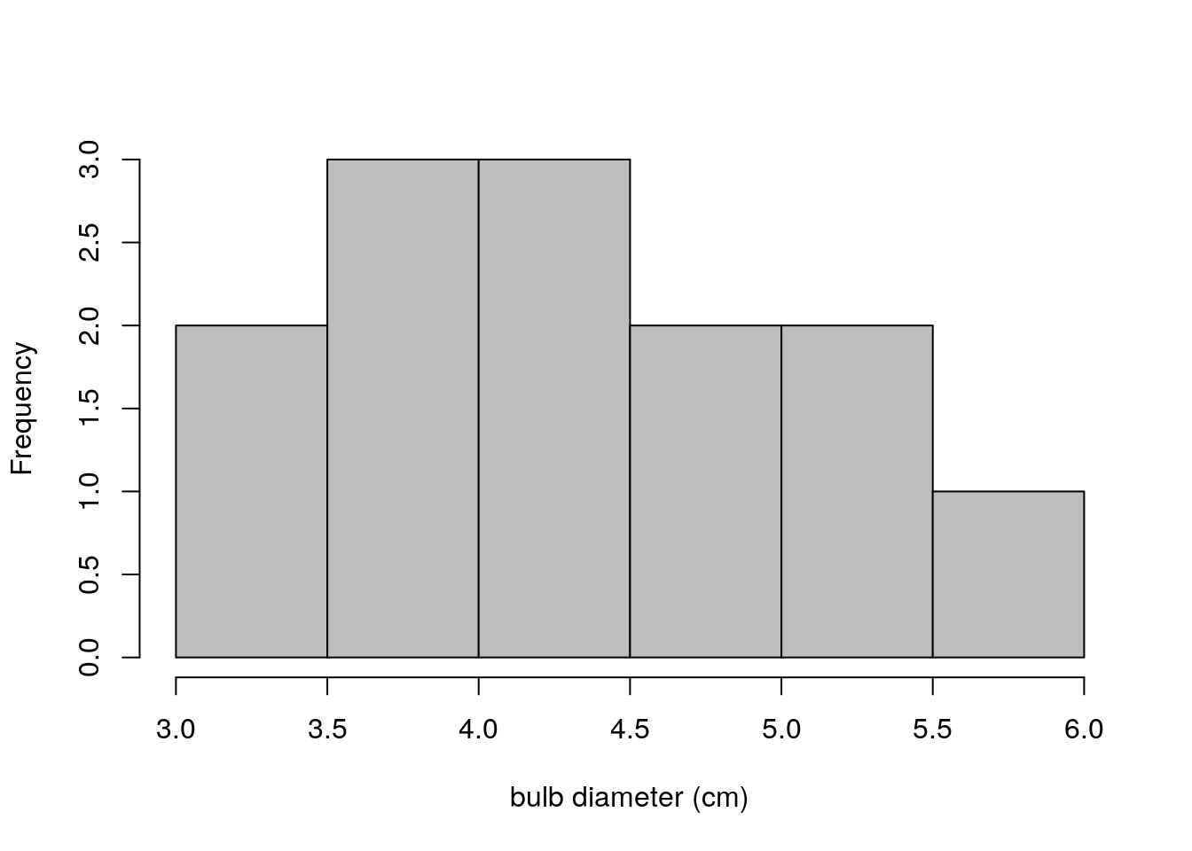
Figure 2.1: Bulb diameters from first sample of 13 turnips
This distinction cannot be emphasized enough. The plot immediately above (figure 2.3) shows bulb diameters of 13 individual turnips. The previous two plots showed means and standard deviations calculated from 5 samples of turnips, where each sample had 13 turnips in it. This is the distinction between a distribution of data and a sampling distribution of a statistic. A distribution of data is exactly what it sounds like. A sampling distribution of a statistic is the distribution of values that statistic takes on, under (perhaps hypothetical) repeated sampling.
Compare the sampling distribution of standard deviations (figure 2.2) to the distribution of raw bulb diameters (figure 2.3). The plot of standard deviations of bulb diameters shows values ranging between 0.75 and 1.05. The plot of just bulb diameters shows values ranging between 3.0 and 6.0. Clearly these are not plots of the same kind of quantity! Recall that our population standard deviation is \(\sigma=0.92\), so it makes sense that the sample standard deviations for our 5 samples would be between 0.75 and 1.05.
So, we have made sampling distributions for two kinds of common statistics (means and standard deviations). But, these sampling distributions are incomplete; we only took five samples! To simulate a sampling distribution in a way that is useful, we should be taking a lot of repeated samples. We’ll start with 10,000. (The more the better; a sampling distribution in principle is the distribution of a statistic calculated over an infinite number of samples).
Important: note the distinction between sample size (n=13 turnips per sample) and number of samples taken (some arbitrarily large number). Do not confuse the two! N=13 is not “the number of samples”. It’s the number of observations (or data points) in the sample.
Here’s a way of simulating sampling distributions of the mean and standard deviation of bulb diameter when n=13.
reps <- 1e4
bulb_means <- rep(0,reps)
bulb_std_devs <- rep(0,reps)
for (i in 1:reps) {
  this_sample <- rnorm(n=13,mean=4.3,sd=0.92)
  bulb_means[i] <- mean(this_sample)
  bulb_std_devs[i] <- sd(this_sample)
}
reps <- 1e4 establishes the number of repeated samples we will take.
1e4 means \(1*10^4\)
bulb_means <- rep(0,reps) creates a vector of 10,000 zeroes. These zeroes will be replaced by the means for all 10,000 samples as the loop repeats.
for (i in 1:reps) {...} Tells R to run the code in brackets 10,000 times, each time increaing the value of i by 1.
this_sample <- rnorm(n=13,mean=4.3,sd=0.92) draws 13 values at random from a \(Normal\ (\mu=4.3,\sigma=0.92)\) distribution and assigns them to the vector this_sample
bulb_means[i] <- mean(this_sample) takes the mean of these 13 values and assigns them to the \(i^{th}\) entry in bulb_means. This happens 10,000 times.
Time to take a look!
hist(bulb_means)
Figure 2.2: Simulated sampling distribution of mean bulb diameter. Each sample is size n=13, and 10,000 repeated samples were taken.
hist(bulb_std_devs)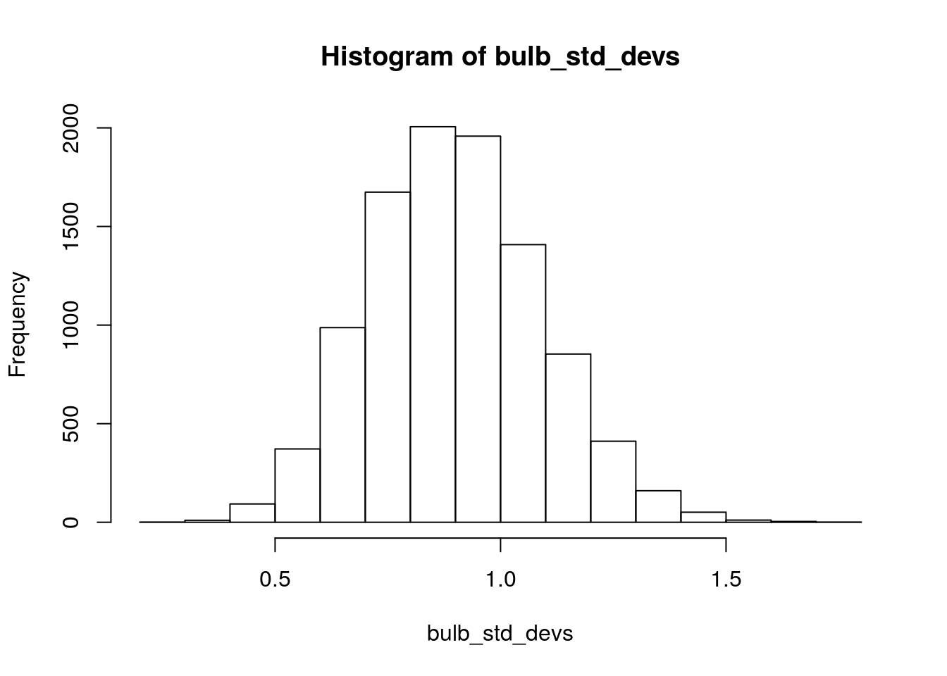
Figure 2.3: Simulated sampling distribution of standard deviation of bulb diameter. Each sample is size n=13, and 10,000 repeated samples were taken.
2.3 Using the sampling distribution to estimate standard error
The standard error of a statistic is defined as the standard deviation of its sampling distribution. We just simulated a sampling distribution for mean bulb diameter (\(n=13\)); let’s get its standard deviation:
sd(bulb_means)## [1] 0.2539848This is our simulated standard error for sample mean bulb diameter when \(n=13\). It is an approximation for the population (or “true”) standard error for sample mean bulb diameter, again when \(n=13\).
The “true” standard error has a formula:
\[ se( \bar{x} )=\frac{\sigma_x}{\sqrt{n}}=\frac{0.92}{\sqrt{13}}=0.255 \]
Well, isn’t that nice? The formula for the standard error of \(\bar{x}\) gives us nearly the same number as we got from taking the standard deviation of our simulated sampling distribution of \(\bar{x}\).
The “standard error” gets it name from the fact that we use statistics (values calculated from data) to estimate parameters (values that are unknown but assumed to exist at the population level). Our estimates will always be wrong by some amount. Call this “some amount” the error in our estimates. The standard error is the standard amount by which we expect our estimates will be in error (so long as the “error” is all due to chance and the sampling distribution is centered on the true parameter value).
Put differently, the standard deviation of data is the standard amount by which those data deviate from their mean. The standard error is the standard amount by which a statistic deviates from the population parameter it is estimating.
We can also use our simulated sampling distribution of the standard deviation to approximate the standard error of the sample standard deviation when \(n=13\):
sd(bulb_std_devs)## [1] 0.1897487Take another look at the histogram of bulb_std_devs, and see if this seems like a reasonable value for the standard deviation of this sampling distribution.
2.4 Using the sampling distribution to test against a null hypothesis
Now that we’ve seen what sampling distributions are, we’ll take a look at how they connect to the interpretation of the p-value.
Suppose we take a sample of \(n=13\) turnips grown using a different fertilizer. We calculate a mean bulb diameter of \(\bar{x}=4.8\)cm. We are wondering whether these turnips came from a population whose mean bulb diameter is larger than that of the previous fertilizer, which had a mean of \(\mu=4.3\) (we’ll just pretend, unrealistically, that we know this parameter value).
Well, we have our simulated sampling distribution for mean bulb diameter when taking samples of size \(n=13\) of turnips grown using the first fertilizer:
hist(bulb_means)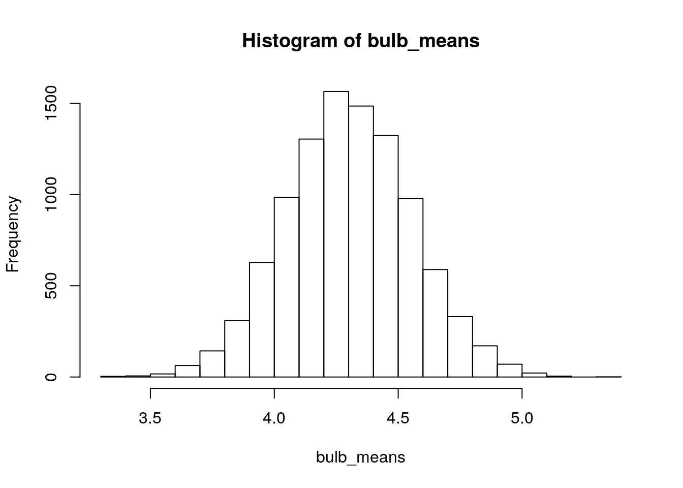
Does \(\bar{x}=4.8\) seem like the kind of mean we’d expect to get from this sampling distribution? Let’s just check to see how often we got sample means at least this big when we simulated them:
sum(bulb_means>4.8)## [1] 269We simulated 10,000 samples, so the proportion of sample means greater than 4.8 was \(\frac{267}{10000}=0.0267\). This is our approximate (simulated) p-value that tests the null hypothesis that the population mean bulb diameter for the new fertilizer is 4.3cm (\(H_0:\mu=4.3\)) against the alternative hypothesis that the population mean bulb diameter for the new fertilizer is larger than 4.3cm (\(H_1:\mu>4.3\)). 10
You may recall the formula for a one-sample z-test when \(\sigma\) is known 11. Let’s see what that gives us: \[ z=\frac{\bar{x}-\mu_0}{\frac{\sigma}{\sqrt{n}}}=\frac{4.8-4.3}{\frac{0.92}{\sqrt{13}}}=\frac{0.5}{0.255}=1.961 \] If our data came from a normal distribution, this z-statistic follows the “standard normal” z-distribution, so we can compute \(P(z>1.961)\):
pnorm(1.961,lower.tail = FALSE)## [1] 0.02493951Well how about that?! Our simulated sampling distribution gave us the approximate probability of getting \(\bar{x}>4.8\) when our data come from a normal distribution with \(\mu=4.3\) and \(\sigma=0.92\), using a sample size of \(n=13\)… and we didn’t need to use R to calculate a probability from the normal distribution, except to check our work!
2.5 Using simulation to conduct a two-sample t-test
Now let’s suppose we’ve collected two samples of turnips, one for each type of fertilizer. The classic two-sample t-test (called “Student’s t-test”) assumes that the data from each group came from a normally distributed population and that the populations have the same variance (variance is standard deviation squared, or \(\sigma^2\)). The null hypothesis says that their means are also the same.
So, if we have fertilizers A and B, our data generating mechanism is:
\[ X_{Ai}\sim Normal(\mu_A,\sigma), i=1, 2, ..., n_A\\ X_{Bi}\sim Normal(\mu_B,\sigma), i=1, 2, ..., n_B \] Here,
- \(X_{Ai}\) is the bulb diameter for the \(i^{th}\) turnip given fertilizer A
- \(X_{Bi}\) is the bulb diameter for the \(i^{th}\) turnip given fertilizer B
- \(n_A\) and \(n_B\) are the sample sizes for the two respective fertilizers
- \(\mu_A\) and \(\mu_B\) are the population mean diameters for bulbs grown with the two respective fertilizers
- \(\sigma\) is the population standard deviation of bulb diameters. Note that this value has no subscript; it is the same for both fertilizers.
The standard null hypothesis would be \(H_0:\mu_A-\mu_B=0\), equivalent to \(H_0:\mu_A=\mu_B\)
Let’s simulate data from a single run of this hypothetical experiment, using equal sample sizes and assuming that the means differ by 0.25cm:
set.seed(335)
N=13
diameters_A <- rnorm(n=N,mean=4,sd=0.92)
diameters_B <- rnorm(n=N,mean=4.25,sd=0.92)
boxplot(diameters_A,diameters_B,names=c("A","B"))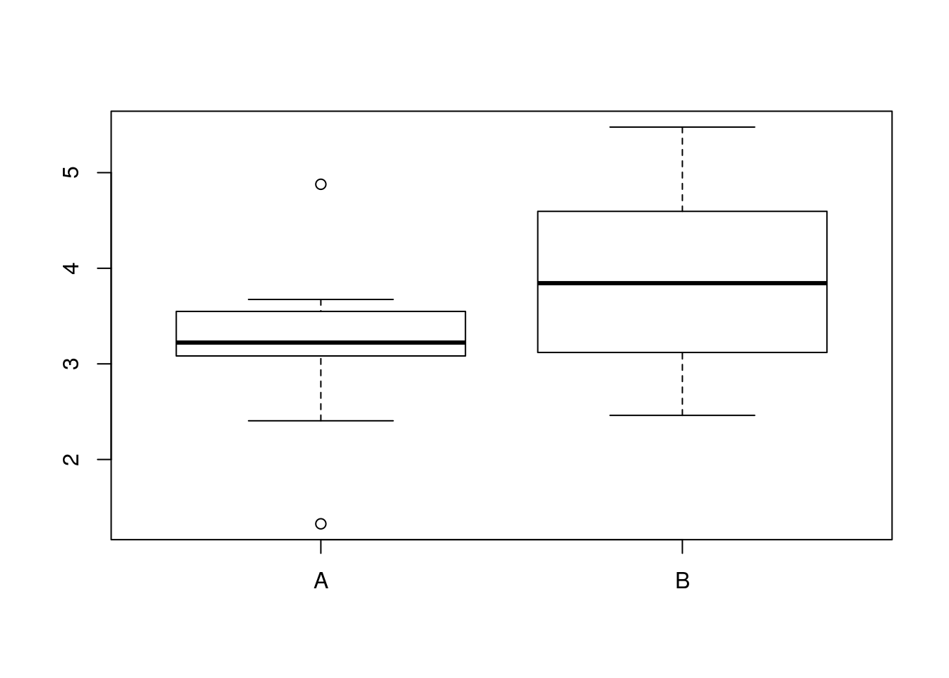
bulb_mean_difference <- mean(diameters_A)-mean(diameters_B)
bulb_mean_difference
## [1] -0.610914So, now we have a simulated sample and a resulting difference in mean bulb diameter.
There is one more complication. In the previous example, we made the unrealistic assumption that the population standard deviation, \(\sigma\), was known. This allowed us to use a z-test statistic, which contains \(\sigma\) in the denominator. The t-test statistic uses sample standard deviation rather than population standard deviation. Here is Student’s t-test statistic:
\[ \begin{split} t&=\frac{\bar{x_1}-\bar{x_2}}{s_p\sqrt{\frac{1}{n_1}+\frac{1}{n_2}}}\hspace{1cm} df=n_1+n_2-2 \\ \\where\quad s_p&=\sqrt{\frac{(n_1-1)s_1^2+(n_2-1)s_2^2}{n_1+n_2-2}} \end{split} \] When group sample sizes are equal (so that \(n_1=n_2=n\)), this simplifies to:
\[ \begin{split} t&=\frac{\bar{x_1}-\bar{x_2}}{\sqrt{\frac{1}{n}(s_1^2+s_2^2)}}\hspace{1cm} df=2n-2 \end{split} \]
So, we’ll simulate the sampling distribution of this test statistic, under the null hypothesis, by drawing repeated samples from normal distributions with the same means and variances and calculating the t-statistic each time.12
For the sake of precision, we’ll use 100,000 reps (1e5) rather than 10,000 reps (1e4). Increasing reps presents a trade-off between the precision of simulated values and the time it takes to run the simulation. For this simulation, calculating the t-statistic doesn’t take much computing power.
reps <- 1e5
N=13
t_statistics_null <- rep(0,reps)
for (i in 1:reps) {
  bulbs_A <- rnorm(n=N,mean=4.5,sd=0.92)
  bulbs_B <- rnorm(n=N,mean=4.5,sd=0.92)
  t_statistics_null[i] <- (mean(bulbs_A)-mean(bulbs_B))/sqrt((sd(bulbs_A)^2+sd(bulbs_B)^2)/N)
}
hist(t_statistics_null)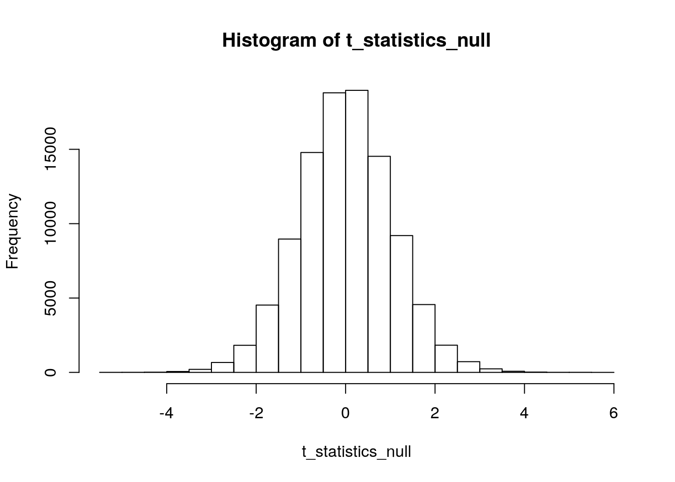
The “observed” mean difference from our simulated data was -0.6109. But, to get a p-value using our simulated distribution under the null, we need to turn this into a t-test statistic:
sd(diameters_A)## [1] 0.7935559sd(diameters_B)## [1] 0.8921635\[ t=\frac{-0.619}{\sqrt{\frac{1}{13}(0.7936^2+0.8922^2})}=\frac{-0.6109}{0.3312}=-1.8445 \] Let’s see how often we get a t-test statistic at least this extreme (in either direction) under our simulated null distribution. We’ll use ‘abs()’ to take the absolute values of our differences under the null and our “observed” difference, so that we are counting up how often a value under the null distribution is “more positive” than 1.8445 or “more negative” than -1.8445:
sum(abs(t_statistics_null)>abs(-1.8445))## [1] 7748We have 7,748 instances of a difference “more extreme” than \(t=-1.8445\) under our simulated null distribution. And, we used 100,000 reps to make this distribution. So, our simulated p-value is 0.07748.
To find our two-sided p-value using the theoretical t-distribution, we need to calculate \(P(T<-1.8445)+P(T>1.8445)\):
pt(-1.8445,df=24,lower.tail = T) + pt(1.8445,df=24,lower.tail = F)## [1] 0.07748875Hooray! This is the same p-value that we got from our simulated null distribution.
While we’re at it, let’s just see what t.test() gives us…
t.test(diameters_A,diameters_B,var.equal = T)##
## Two Sample t-test
##
## data: diameters_A and diameters_B
## t = -1.8448, df = 24, p-value = 0.07745
## alternative hypothesis: true difference in means is not equal to 0
## 95 percent confidence interval:
## -1.29439859 0.07257051
## sample estimates:
## mean of x mean of y
## 3.202399 3.813313There’s our p-value! Here’s how to get just the p-value:
t.test(diameters_A,diameters_B,var.equal = T)$p.value## [1] 0.07744969One more go, just to make sure this works…
set.seed(42)
N=13
diameters_A <- rnorm(n=N,mean=4,sd=0.92)
diameters_B <- rnorm(n=N,mean=4.25,sd=0.92)

(mean(diameters_A)-mean(diameters_B))/sqrt((sd(diameters_A)^2+sd(diameters_B)^2)/N)
## [1] 1.200844sum(abs(t_statistics_null)>abs(1.200844))/1e5## [1] 0.24417pt(-1.200844,df=24,lower.tail = T) + pt(1.200844,df=24,lower.tail = F)## [1] 0.2415298t.test(diameters_A,diameters_B,var.equal = T)$p.value## [1] 0.2415299Our “simulated” p-value is off by 0.0026. We can probably live with this. If we wanted less error, increase the number of reps used to create the simulated null distribution would get us closer to the “real” p-value.
2.6 Using simulation to check Type I error rate
To recap what we just did:
- We generated fake data according to the assumptions of our statistical procedure, and calculated an “observed” test statistic.
- We generated a “null distribution” of values that this test statistic will take on when the null hypothesis is true.
- We confirmed that the p-value we get from using
t.testorpt()is the same one we get from finding the proportion of test statistics under our simulated null distribution that are greater than the one we observed.
What was the point of this?
- To emphasize the “under repeated sampling” aspect of the p-value’s interpretation. The p-value is the answer to the question: “how often would I get a result at least as extreme as mine if the null were true and I kept doing the same study over and over again using new random samples from the same population?”
- To show that the statistic \(\frac{\bar{x_1}-\bar{x_2}}{\sqrt{\frac{1}{n}(s^2_1+s^2_2})}\) really does follow the theoretical t-distribution, provided some assumptions are met.
- To show how simulation can be used to investigate properties the of a statistical procedure.
Here’s another important property of hypothesis testing: if our rule is to reject \(H_0\) when \(p < \alpha\), then when \(H_0\) is true, we will reject it with probability \(\alpha\). This is the “Type I error rate”:
\[ P(reject\ H_0|H_0\ true)=\alpha \]
Well, let’s check to see if we get this rate using simulation! We’ll repeatedly generate new samples under the null hypothesis, save the p-values, and see how often we get \(p<\alpha\). (We’ll use \(\alpha=0.05\), because that’s what everyone else uses.)
set.seed(335)
reps <- 1e4
pvals <- rep(0,reps)
for (i in 1:reps) {
  sample_1 <- rnorm(n=67,mean=20,sd=4)
  sample_2 <- rnorm(n=67,mean=20,sd=4)
  pvals[i] <- t.test(sample_1,sample_2,var.equal = T)$p.value
}
sum(pvals<0.05)/reps
## [1] 0.0488Close enough! It should be 0.05, but we only used 10,000 reps for this simulation. Using more reps would get us a little closer.
Since we just make a sampling distribution of the p-value when \(H_0\) is true, let’s see what it looks like…
hist(pvals)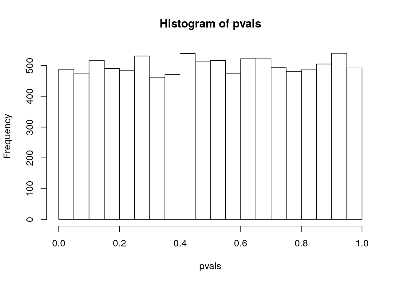
It turns out that the sampling distribution of the p-value is, for most tests, uniform under \(H_0\). This means that every p-value has the same probability of occurring as every other p-value, if the null hypothesis is true.
2.7 Using simulation to break the rules
In chapter 8, we’ll use simulation to take a close look at what happens when modeling assumptions are violated. For now, here’s a quick example.
Remember that the classic t-test assumes that our two populations have the same variance? Let’s simulate p-values when \(H_0:\mu_1 - \mu_2=0\) is true but the variances aren’t equal, and see what happens. Here, we’ll use \(\sigma_1=2\) and \(\sigma_2=10\):
set.seed(335)
reps <- 1e4
pvals <- rep(0,reps)
for (i in 1:reps) {
  sample_1 <- rnorm(n=67,mean=20,sd=2)
  sample_2 <- rnorm(n=67,mean=20,sd=10)
  pvals[i] <- t.test(sample_1,sample_2,var.equal = T)$p.value
}
sum(pvals<0.05)/reps
## [1] 0.0485Well, that’s not so bad, maybe even within the error tolerance we expect from simulation. Ok, now let’s do it with unequal sample sizes of \(n=47\) and \(n=87\):
reps <- 1e4
pvals <- rep(0,reps)
for (i in 1:reps) {
  sample_1 <- rnorm(n=87,mean=20,sd=2)
  sample_2 <- rnorm(n=47,mean=20,sd=10)
  pvals[i] <- t.test(sample_1,sample_2,var.equal = T)$p.value
}
sum(pvals<0.05)/reps
## [1] 0.148Yikes! Our Type I error rate is now almost 3 times too big!
Now, let’s keep the unequal sample sizes but make the variances the same again:
reps <- 1e4
pvals <- rep(0,reps)
for (i in 1:reps) {
  sample_1 <- rnorm(n=87,mean=20,sd=4)
  sample_2 <- rnorm(n=47,mean=20,sd=4)
  pvals[i] <- t.test(sample_1,sample_2,var.equal = T)$p.value
}
sum(pvals<0.05)/reps
## [1] 0.0485And, we’re back to normal. It turns out that the “equal variance” assumption can be violated pretty heavily without affecting the Type I error rate, so long as the sample sizes are equal. And the sample sizes can be unequal, so long as the other assumptions are met. But violating assumptions and having unequal sample sizes can wreak havoc. And we just saw this very quickly, using simulation. Simulation is a great tool for discovering exactly what happens when you “break the rules”. Sometimes the consequences are serious; sometimes they are trivial.
Remember how we’ve been using the “classic” t-test, called Student’s t? The var.equal=T argument in t.test() tells R to use Student’s t. But, R actually defaults to using a different t-test, called “Welch’s t”. And for good reason: Welch’s t doesn’t assume equal variances!
Let’s run the same simulation code that got us a Type I error rate of 0.148 above, but this time removing the var.equal=T argument:
reps <- 1e4
pvals <- rep(0,reps)
for (i in 1:reps) {
  sample_1 <- rnorm(n=87,mean=20,sd=2)
  sample_2 <- rnorm(n=47,mean=20,sd=10)
  pvals[i] <- t.test(sample_1,sample_2)$p.value
}
sum(pvals<0.05)/reps
## [1] 0.0488A lesson from this simulation: don’t use Student’s t 13.
2.8 Simulating 95% confidence intervals
We could do this using R code, but this website’s simulation is beautiful:
“Seeing Theory” confidence interval simulation, Brown University
The main lesson here is that, under repeated sampling, confidence intervals capture the unknown parameter value \((1-\alpha)*100\%\) of the time. For example, if \(\alpha = 0.10\), repeatedly creating confidence intervals should result in the true parameter being captured \((1 - .1) * 100\% = 90\%\) of the time.
2.9 Connecting confidence intervals and hypothesis tests
We will compare the “estimation” and “testing” approaches to inference in detail in module 4. For now, we’ll just note how confidence intervals and hypothesis tests are connected.
Mathematically, a confidence interval is constructed by “inverting” a hypothesis test to find all of the possible null values that would not be rejected by our data.
Specifically, a \((1-\alpha)*100\%\) confidence interval contains all of the values that would produce \(p > \alpha\) if tested against. And, all of the values outside of a \((1-\alpha)*100\%\) confidence interval would produce \(p<\alpha\) if tested against.
For example, if we have data that gives us \(95\%\ CI\ for\ \mu_1-\mu_2=(-2.3,-0.7)\), we know that using these same data to test \(H_0:\mu_1-\mu_2=0\) will give a p-value less than 0.05 (and so we will reject \(H_0\)).
We also know that testing \(H_0:\mu_1-\mu_2=-1\) will give a p-value greater than 0.05 (fail to reject \(H_0\)), and that testing \(H_0:\mu_1-\mu_2=-3\) will give a p-value less than 0.05, and so on. Testing against any value inside this interval will result in failing to reject \(H_0\); testing against any value outside it will result in rejecting \(H_0\).
Bringing this back to the Type I error rate, suppose that a null hypothesis \(H_0:\mu_1-\mu_2=0\) is true. Under repeated sampling, \(95\%\) of all \(95\%\) confidence intervals will capture the true parameter value of zero. And so \(5\%\) of \(95\%\) confidence interval will not capture zero. If the confidence interval does not capture zero, we reject \(H_0:\mu_1-\mu_2=0\). And so, a \(95\%\) confidence interval implies a \(5\%\) Type I error rate.
We noted at the beginning of the module that the “confidence” we have in confidence intervals comes from their long run success rate: a \(95\% CI\) captures the unknown parameter value \(95\%\) of the time. We could also say that our “confidence” comes from the fact that the interval contains all values that our data would not reject. In this sense, a confidence interval contains all of the possible parameter values that would be reasonably likely to produce data like ours.
2.10 “Repeated sampling” is (usually) a thought experiement
Classical inference appeals to the properties of our methods, “under repeated sampling”. For instance, we have “confidence” in our confidence interval because it was made using a method that usually works, “under repeated sampling”. We should probably say “under hypothetical repeated sampling”, because we almost never actually do repeated sampling. We have our one sample, and from it we calculate one confidence interval. We justify our confidence in the interval by saying that the method we used would have a 95% success rate if we were keep taking new samples and kept making new confidence intervals, over and over and over again.
This does not mean that we are obligated to keep taking new samples, or that our inferences only make sense if we keep taking new samples. Our inferences refer to a thought experiment. We imagine a hypothetical scenario in which we keep taking new samples. If we accept that, under this hypothetical scenario, 95% of these samples would produce confidence intervals that contain the unknown value of interest, then we can feel “confident” that the one actual confidence interval we made contains this value. After all, it’s more likely that our sample is one of the 95% of (hypothetical) samples in which the interval succeeds than one of the 5% in which it doesn’t.
This applies to p-values as well. The interpretation of the p-value also requires a thought experiment: if we lived in the world in which the null hypothesis is true, and if we could keep taking new samples from the sample population over and over again and computing a new test statistic each time, the p-value is the proportion of these hypothetical new samples that would produces test statistics larger than the one we actually calculated from our one actual sample. In other words, a small p-value tells you that the test statistic you actually got is bigger than what you’d usually get under the hypothetical scenario where the null is true and you could keep doing this study over and over again with new data each time.
2.11 List of common misconceptions about p-values and confidence intervals
The purpose of this module was to lay down the foundation for classical inference, and to show how simulation can be used to investigate the properties of statistical methods “under repeated sampling”.
As we will see in the next module, there is some controversy over classical methods, particularly over the use of p-values and hypothesis testing. And, there are common misconceptions and misinterpretations that we will briefly address now.
This 2016 paper covers a wide array of misinterpretations of p-values and confidence intervals. (Greenland et al. 2016). Note that this paper refers to the “test hypothesis”, which is the hypothesis we are testing against; we also call this the “null hypothesis”. Some very common ones (remember, these are all false):
- The P value is the probability that the test hypothesis is true; for example, if a test of the null hypothesis gave P = 0.01, the null hypothesis has only a 1% chance of being true; if instead it gave P = 0.40, the null hypothesis has a 40% chance of being true.
- The P value for the null hypothesis is the probability that chance alone produced the observed association; for example, if the P value for the null hypothesis is 0.08, there is an 8% probability that chance alone produced the association.
- A null-hypothesis P value greater than 0.05 means that no effect was observed, or that absence of an effect was shown or demonstrated.
- If you reject the test hypothesis because P < 0.05, the chance you are in error (the chance your “significant finding” is a false positive) is 5%.
- Statistical significance is a property of the phenomenon being studied, and thus statistical tests detect significance.
- When the same hypothesis is tested in two different populations and the resulting P values are on opposite sides of 0.05, the results are conflicting.
- The specific 95% confidence interval presented by a study has a 95% chance of containing the true effect size.
- An observed 95% confidence interval predicts that 95% of the estimates from future studies will fall inside the observed interval.
A 2002 study found high rates of endorsements of incorrect interpretations of p-values among students and teachers of statistical methods. (Haller and Krauss 2002).
A 2014 study found similarly high rates of endorsements of incorrect interpretations of confidence intervals among PhD researchers, graduate students, and first-year undergraduates. On some interpretations, PhD researchers performed more poorly than first-year undergraduates. (Hoekstra et al. 2014)
A 2016 study found that over half of students or researchers with statistical training will say that numbers which are different from one another are “no different” from one another, if the numbers are accompanied by “P > 0.05”. (Blakeley B. McShane and Gal 2016) Unsurprisingly, undergraduate college students with no statistical training correctly identified numbers that are different from one another as being different from one another at very high rates. (The worst performing group in this study were editorial board members at a major journal.)
A 2020 study found misinterpretations of significance in 89% of introductory psychology textbooks surveyed (Cassidy et al. 2019). I haven’t seen similar studies done for other fields, but I can say from experience that I’ve read plenty of similar misinterpretations in biology and economics textbooks as well.
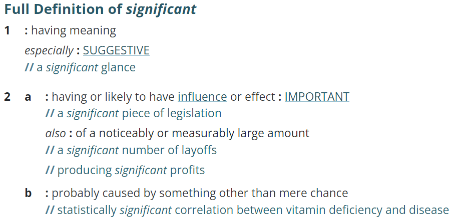
Even Merriam-Webster gets it wrong!
References
We will explore the distinction between frequentist and Bayesian approaches in the next module.↩︎
Here, “justified” means “supported” or “backed up”; you are under no obligation to find these justifications compelling↩︎
This line of reasoning is controversial; we will explore some debates surrounding hypothesis testing and statistical significance in the next two modules.↩︎
This is the kind of thing that Ronald Fisher, popularizer of p-values and statistical significance in the early 1900s, did a lot of.↩︎
This is known as a “one-sided” p-value↩︎
\(\sigma\) is never known↩︎
It isn’t clear what value to use as the population mean here, but thankfully this doesn’t matter; we’re going to use the same mean for both groups and so their population difference will be zero regardless of what value we choose for the mean.↩︎
Seriously, there’s just no good reason to use Student’s t rather than Welch’s t. Best case scenario, they give you the same result.↩︎