3 Bayesian vs. frequentist probability
In the previous module, we looked at the reasoning behind frequentist inference. In this module, we will introduce Bayesian inference, and explore how frequentist and Bayesian approaches differ.
3.1 Relative frequency
3.1.1 Quick recap
A quick summary of the main points from the previous module:
The frequentist approach treats probabilities as relative frequencies. If we say that the probability of rolling a 5 on a fair die is \(\frac{1}{6}\), we mean that, if the die were rolled an infinite number of times, \(\frac{1}{6}^{th}\) of all rolls would be a 5. More practically, if we roll the die a large (but non-infinite) number of times, we will predict (or “expect”) \(\frac{1}{6}^{th}\) of our rolls to land on 5.
If we say the probability of getting a test statistic at least as large as \(z=\pm 1.96\) under a null hypothesis is \(0.05\), what we mean is that, if could take an infinite number of samples from the same population and the null hypothesis is true, then we will get \(|𝑧|\geq 1.96\) 1 out of every 20 times.
If we say that a \(95\%\) CI has \(95\%\) coverage probability for a parameter \(\theta\), what we mean is that, if we could take an infinite number of samples from the same population, our method would produce an interval that contains \(\theta\) in 19 out of every 20 samples.
Frequentist probability is sometimes thought of as “physical” probability, because it quantifies rates of outcomes in physical processes that we are willing to characterize as random.
3.1.2 What frequentism does not allow
Frequentist probabilities can only be assigned to random variables.
Data are considered random (“we took a random sample of…”). Statistics are calculated from data, and so statistics are considered random variables. We can make probability statements about the values that statistics will take on.
Hypotheses are not random. Parameters are not random. “The truth” is not random. Frequentist probabilities cannot be assigned to these.
This might explain why frequentist interpretations sometimes feel strange: we must always be careful to direct our probability statements at statistics or data, and not at hypotheses or parameters.
Examples:
We cannot talk about “the probability that the null hypothesis is true”, because the truth value of the null hypothesis is not random. The null is either true or false. Just because we don’t know whether it is true or false does not make whether it is true or false a random variable. Instead, we talk about the probability of getting some kind of statistical result if the null is true, or if the null is false.
We cannot talk about the probability that a parameter’s value falls inside a particular confidence interval. The parameter’s value is not a random variable. And once data have been collected, the “random” part is over and the confidence interval’s endpoints are known. There is now nothing random going on. Either the parameter value is inside the interval or it is outside the interval. The fact that we don’t know the parameter’s value does not make its value a random variable. Instead, we talk about the probability that a new random sample, not yet collected, would produce a confidence interval that contains the unknown parameter value.
3.2 Degrees of belief
The Bayesian approach treats probability as quantifying a rational degree of belief. This approach does not require that variables be “random” in order to make probability statements about their values. It does not require that probabilities be thought of as long run relative frequencies14.
Here are some probabilities that do not make sense from the frequentist perspective, but make perfect sense from the Bayesian perspective:
The probability that a hypothesis is true.
The probability that \(\mu_1-\mu_2\) falls inside a 95% confidence interval that we just computed (though Bayesians call their intervals “credible” intervals)
The probability that a fever you had last week was caused by the influenza virus.
The probability that the person calling you from an unknown telephone number wants to sell you something.
The probability that an election was rigged.
The probability that a witness testifying in court is lying about how they first met the defendant.
These probabilities do not refer to frequencies15. They refer to how much belief one is willing to apply to an assertion.
The mathematics of probabililty work the same in the Bayesian approach as they do in the frequentist approach. Bayesians and frequentists sometimes choose to use different mathematical tools, but there is no disagreement on the fundamental laws of mathematical probability. The disagreement is on what statistical methods to use, and how to interpret probabilistic results.
3.2.1 Bayes doesn’t need randomness
The Bayesian approach does not require anything to be random. Pierre-Simon Laplace, who did work on mathematical probability and who used the Bayesian approach to inference, believed that the universe was deterministic:
We may regard the present state of the universe as the effect of its past and the cause of its future. An intellect which at a certain moment would know all forces that set nature in motion, and all positions of all items of which nature is composed, if this intellect were also vast enough to submit these data to analysis, it would embrace in a single formula the movements of the greatest bodies of the universe and those of the tiniest atom; for such an intellect nothing would be uncertain and the future just like the past would be present before its eyes.
Laplace did not believe in true randomness, but still embraced probability as a valuable tool for dealing with the unknown.
Let’s relate this idea directly to statistical inference. From a frequentist perspective, there is no such thing as the probability that a null hypothesis is true (unless that probability is zero or one). The null is either true or it is not; its truth value is not random. But from a Bayesian perspective, it is fine to assign a probability to the null being true, because we do not know whether it is true. That probability will quantify the strength of our belief that the null is true, and Bayesian methods use data to inform that strength of belief.
3.3 Priors and updating
Does this all sound wonderful and amazing? Are you excited to learn that, despite what we saw in module 2, statistics can be used quantify the probability that a hypothesis is true, or the probability an unknown value lies inside the interval we calculated?
Well, there is one more important element to Bayesian inference, and it complicates thing: priors.
“Priors” refer to beliefs held prior to your data analysis, or information known before your data analysis. They take the form of probabilities.
- A prior can be a single probability of some statement being true. Examples: the prior probability that a null hypothesis is true; the prior probability that a witness in court is lying.
- A prior can be a probability distribution, which assigns probabilities to all the values that a variable might take on. Example: the prior distribution for the effectiveness of a Facebook ad on ticket sales for concerts, defined as the % change in tickets sold when comparing concerts that are advertised on Facebook to those that are not. Such a prior distribution might look like this:
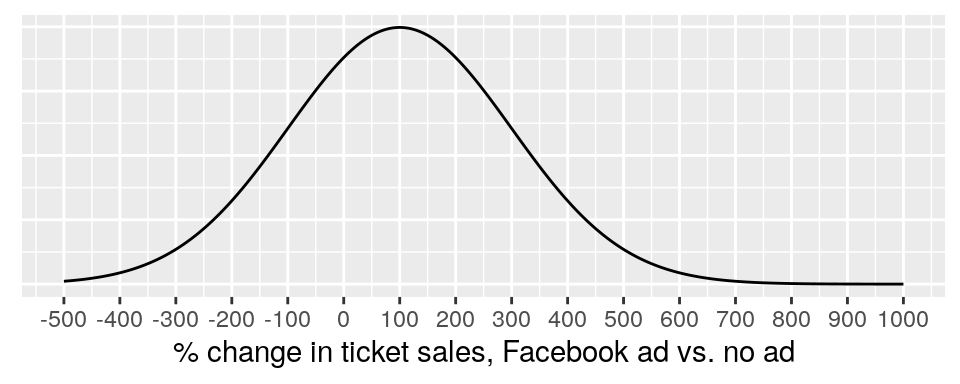
This is showing a prior probability distribution for \(P(effectiveness)\), defined as \(Normal(\mu=100,\sigma=200)\) This is a fairly weak prior distribution: it is centered on 100% (or a doubling of sales), but it has a standard deviation of 200, thus allowing some prior probability for unlikely values (300% decrease; 600% increase).
A stronger prior might look like this:
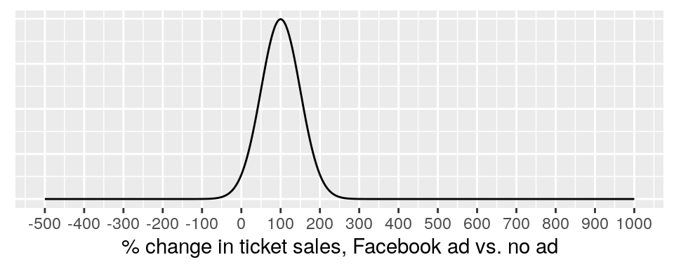
This is a “stronger” prior distribution than before, because it is effectively ruling out the extreme possibilities for changes in ticket sales.
We might also choose a distribution other than normal, since it seems unlikely that the ad will reduce sales. Maybe we find a distribution that has a long right tail, giving some probability that the ad will have a huge positive effect on sales, but also a short left tail, giving very little probability to the ad being counterproductive to a large degree.
A prior is effectively a probability “starting point” that you set before seeing data. The data are then combined with the prior to “update” the beliefs or information contained in the original prior, giving a “posterior”.
Priors are essential to Bayesian inference. If we want to make probability statements about parameters or hypotheses using data, we need to establish our starting point.
Some people argue that priors are a desirable feature in statistical inference, because they allow us to formally include information from beyond our data into our analyses. Others argue that priors undermine statistical inference, because they are inherently subjective. How can I say I’m making conclusions based on the data if those conclusions are also affected by the prior I chose? How can we trust the results of a data analysis when two people using the same method but different priors get different results?
More on that later. It’s time now to take a look at “Bayes’ Rule”
3.4 Bayes’ Rule
Behold!
\[ P(B|A)=\frac{P(A|B)P(B)}{P(A)} \] In Bayesian statistics, we are typically drawing inference on parameters, using data. Call the parameter vector \(\boldsymbol{\theta}\) and the data matrix \(\textbf{X}\):
\[ P(\boldsymbol{\theta}|\textbf{X}) =\frac{P(\textbf{X}|\boldsymbol{\theta})P(\boldsymbol{\theta})}{P(\textbf{X})} \] Where
- \(P(\boldsymbol{\theta}|\textbf{X})\) is the posterior probability distribution of the parameters
- \(P(\textbf{X}|\boldsymbol{\theta})\) is the likelihood of the data, given the parameters
- \(P(\boldsymbol{\theta})\) is the prior probability distribution of the parameters
- \(P(\textbf{X})\) is the total probability of the data
3.4.1 Example: screening test
Suppose that a routine COVID-19 screening test returns a positive result. And, suppose the test has a 2% false positive rate, meaning that if you don’t have COVID-19, there is only a 2 in 100 chance of testing positive. Does this mean that there is a 98% chance that you do have COVID-19?
No. The chance that a person without COVID-19 tests positive is not the same thing as the chance that a person who tests positive has COVID-19:
\[ P(test\ positive\ |\ no\ COVID) \neq P(no\ COVID\ |\ test\ positive) \] The only way to determine \(P(no\ COVID\ |\ test\ positive)\) from \(P(test\ positive\ |\ no\ COVID)\) is to use Bayes’ rule:
\[ P(no\ COVID\ |\ test\ positive)=\frac{P(test\ positive\ |\ no\ COVID)P(no\ COVID)}{P(test\ positive)} \] \(P(no\ COVID)\) is the prior probability of not having COVID-19. How do we decide this value?
- We may use current estimates for the % of the population who have COVID-19 at any given time.
- We may consider “daily life” factors that vary by individual, such as how much time is spent indoors with other people for long periods of time, or whether there’s been a known COVID-19 exposure.
- We may consider whether a person has been infected previously.
- We may consider whether a person has been vaccinated.
- We may simply say we have absolutely no information at all and make the prior 50/50. Such “uninformative” priors are popular.
\(P(test\ positive)\) is the probability that anyone will test positive, whether they have COVID-19 or not. It is the “total probability” of a positive test result.
Let’s suppose that the prior probability of not having COVID-19 is 96%, and that the probability of anyone testing positive is 5%. Then, we have:
\[ \begin{split} P(no\ COVID\ |\ test\ positive)&=\frac{P(test\ positive\ |\ no\ COVID)P(no\ COVID)}{P(test\ positive)} \\ \\ &= \frac{0.02*0.96}{0.05}=0.384 \end{split} \] So, in our hypothetical scenario, we have tested positive using a test that has only a 2% probability of a false positive. And, there is a 38.4% probability that our positive test was a false positive.
3.4.2 Choosing a prior
The most challenging element of the previous example was deciding a prior probability of not having COVID. There seems to be no “objective” way to do this. But although priors are “subjective”, they are not arbitrary. A data analyst using Bayesian tools should be prepared to defend their chosen priors.
In most cases, there is the option to use an “uninformative” prior. Using an uninformative prior can result in a Bayesian analysis producing identical results that a frequentist analysis would produce.
Informative priors don’t need to be very strong. When drawing inference on parameters, priors can be used for the purpose of excluding impossible or extremely unrealistic values, while remaining open to a very broad range of realistic values. Such “weakly informative” priors don’t feel so subjective.
3.4.3 Example: evidence for a crime
Suppose there is a hit and run car accident, where someone causes an accident and then drives off. The victim didn’t see the driver, but did see that the other vehicle was a red truck. Suppose also that 4% of all people drive red trucks.
The police get a tip that someone was overheard at a bar bragging about getting away with running into someone and then driving off. A police officer goes to this person’s house and lo and behold! There’s a red truck in the driveway. Since only 4% of all people drive red trucks, the officer concludes that there is a 96% chance that this person is guilty.
This reasoning is invalid, and common enough to have its own name: the “prosecutor’s fallacy”, or the “base rate fallacy”. The key problem here is the same one we saw in the last example:
\[ P(not\ guilty\ |\ red\ truck) \neq P(red\ truck\ |\ not\ guilty) \] The missing piece of information is the probability of the suspect being guilty prior to seeing the evidence of the red truck. Again, if we are going to assign a probability to a hypothesis using data, we need a starting point!
Let’s say that, based on the police tip, we give this suspect a 20% chance of being guilty prior to us seeing the red truck. Let’s also allow for a 10% probability that the suspect is keeping the red truck somewhere else, out of fear of being caught. Using Bayes’s rule:
\[ \begin{split} P(not\ guilty\ |\ red\ truck)\ &= \frac{P(red\ truck\ |\ not\ guilty)P(not\ guilty)}{P(red\ truck)}\\ \\ \ &=\ \frac{P(red\ truck\ |\ not\ guilty)P(not\ guilty)}{P(red\ truck\ |\ not\ guilty)P(not\ guilty)+P(red\ truck\ |\ guilty)P(guilty)} \\ \\ \ &=\frac{(0.04)(0.8)}{(0.04)(0.8)+(0.90)(0.2)} \\ \\ \ &=0.1509\approx 15\% \end{split} \] We might now be concerned that our posterior probability is heavily influenced by our priors: \(P(not\ guilty)\) and \(P(red\ truck\ |\ guilty)\). A good practice is to try out different values and see how much effect this has on the posterior.
3.4.4 Example: \(P(H_0\ true)\)
We noted in the last chapter that, under frequentist inference, it doesn’t make sense to talk about the probability that a null hypothesis is true. This is because the truth status of the null hypothesis is not a random variable.
For Bayesian inference, this is not a problem. If we want the probability of the null hypothesis being true, given our data, we can use Bayes’ rule. And this means that we must state a prior for \(P(H_0\ true)\)!
\[ \begin{split} P(H_0\ true\ |\ reject\ H_0)&=\frac{P(reject\ H_0\ |\ H_0\ true)P(H_0\ true)}{P(reject\ H_0)} \\ \\ &=\frac{P(reject\ H_0\ |\ H_0\ true)P(H_0\ true)}{P(reject\ H_0\ |\ H_0\ true)P(H_0\ true)+P(reject\ H_0\ |\ H_0\ false)P(H_0\ false)} \\ \\&= \frac{P(Type\ I\ error)P(H_0\ true)}{P(Type\ I\ error)P(H_0\ true)+Power\cdot P(H_0\ false)} \end{split} \] Now, suppose we collect some data and we reject \(H_0\). We are now wondering how likely it is that \(H_0\) is actually true. To do this, we need:
- A prior probability of \(H_0\) being true
- An assumed power for the test, where power is \(P(reject\ H_0\ |\ H_0\ is\ false)\)
Example 1:
Let’s say we choose \(P(H_0)=0.5\) and \(Power=0.8\), and we rejected \(H_0\) at the \(\alpha=0.05\) level of significance, implying \(P(Type\ I\ error)=0.05\). Plugging these values into Bayes’ rule:
\[ \begin{split} &\frac{P(Type\ I\ error)P(H_0\ true)}{P(Type\ I\ error)P(H_0\ true)+Power\cdot P(H_0\ false)} \\ \\&=\frac{0.05\cdot0.5}{0.05\cdot0.5+0.8\cdot0.5}=\frac{0.025}{0.025+0.4}=0.0588 \end{split} \] Oh, hooray! The probability that the null hypothesis is true turns out to be very similar to 0.05, the Type I error rate. So, in this case, \(P(H_0\ true\ |\ reject\ H_0) \approx P(reject\ H_0\ |\ H_0\ true)\). Maybe this always happens!?!?!?!?!?16
Example 2 Let’s suppose that we think the null hypothesis is very likely true, and we assign a prior of \(P(H_0\ true)=0.9\). Let’s also suppose again that power is 0.8:
\[ P(H_0\ true\ |\ reject\ H_0)=\frac{0.05\cdot0.9}{0.05\cdot0.9+0.8\cdot0.1}=\frac{0.045}{0.045+0.08}=0.36 \] Here, our posterior probability of 0.36 for \(H_0\ true\) is substantially smaller than the prior of 0.9, so rejecting \(H_0\) did decrease the probability of \(H_0\) being true. However, the posterior probability for \(H_0\ true\) is much larger than the Type I error rate of \(0.05\). So, rejecting \(H_0\) at \(\alpha=0.05\) absolutely does NOT suggest that the probability of the null being true is close to 0.05.
Example 3 Now let’s suppose we consider the null unlikely to be true, and assign a prior of \(P(H_0\ true)=0.1\). Again using 80% power, we get:
\[ P(H_0\ true\ |\ reject\ H_0)=\frac{0.05\cdot0.1}{0.05\cdot0.1+0.8\cdot0.9}=\frac{0.005}{0.005+0.720}=0.007 \]
Rejecting the already unlikely null substantially reduces its probability of being true.
Example 4 How about when we fail to reject \(H_0\)? We know that \(P(FTR\ H_0\ |\ H_0\ true)=0.95\) and that \(P(FTR\ H_0\ |\ H_0\ false)=1-P(reject\ H_0\ |\ H_0\ false)=1-Power\).
Let’s use the same prior (0.1) and power (0.8) as before:
\[ \begin{split} P(H_0\ true\ |\ FTR\ H_0)&=\frac{P(FTR\ H_0\ |\ H_0\ true)P(H_0\ true)}{P(FTR\ H_0)} \\ \\ &=\frac{P(FTR\ H_0\ |\ H_0\ true)P(H_0\ true)}{P(FTR\ H_0\ |\ H_0\ true)P(H_0\ true)+P(FTR\ H_0\ |\ H_0\ false)P(H_0\ false)} \\ \\&= \frac{P(FTR\ H_0\ |\ H_0\ true)P(H_0\ true)}{P(FTR\ H_0\ |\ H_0\ true)P(H_0\ true)+(1-Power)P(H_0\ false)} \\ \\&= \frac{0.95\cdot 0.1}{0.95\cdot 0.1+0.2\cdot 0.9} \\ \\&= \frac{0.095}{0.095+0.18}=0.345 \end{split} \]
Failing to reject the null increased the probability of the null from 0.1 to 0.345.
Example 5 Finally, let’s look at what happens if we change power. Before performing any calculations, we’ll consider what effect power ought to have on the posterior probability of the null being true.
Suppose we reject \(H_0\). When power is high and \(H_0\) is false, there is a high chance of rejecting \(H_0\). When power is low and \(H_0\) is false, there is a low chance of rejecting \(H_0\). When \(H_0\) is true, there is an \(\alpha=0.05\) chance of rejecting \(H_0\). So, \(P(reject\ H_0\ |\ H_0\ false)\) is nearer to \(P(reject\ H_0\ |\ H_0\ true)=0.05\) when power is low compared to when power is high. Thus, rejecting \(H_0\) when power is low doesn’t provide as much evidence against \(H_0\) as it does when power is high. If we are interested in \(P(H_0\ true\ |\ reject\ H_0)\), rejecting \(H_0\) will reduce \(P(H_0\ true)\) by more in a high power situation than in a low power situation.
Suppose we fail to reject \(H_0\). \(P(FTR\ H_0\ |\ H_0\ true)=0.95\) is more similar to \(P(FTR\ H_0\ |\ H_0\ false)\) when power is low compared to when power is high. Thus, failing to reject \(H_0\) when power is low doesn’t provide as much evidence in support of \(H_0\) as it does when power is high (consider that, when power is high, we are very likely to reject \(H_0\). And so, if we don’t reject \(H_0\), this will shift our belief toward \(H_0\) being true by more than it would if power were low). So, if we are interested in the posterior probability of \(H_0\) being true, we will consider failing to reject \(H_0\) to be stronger evidence in support of \(H_0\) in a high power situaion than in a low power situation.
In either case, the result of a hypothesis test is more informative when power is high than when power is low. Whatever your prior probability is for \(H_0\) being true, the result of a test will move this probability by more in higher power situations. The intuition is that the chances of rejecting vs. failing to reject \(H_0\) are more different from each other when power is high, and so the result of the test should have a greater effect on our belief about the truth or falsity of \(H_0\) when power is high vs. when power is low.
Ok, let’s see how the math shakes out. Here’s the same calculation as in example 4, but with power = 0.3:
\[ \begin{split} P(H_0\ true\ |\ FTR\ H_0)&= \frac{P(FTR\ H_0\ |\ H_0\ true)P(H_0\ true)}{P(FTR\ H_0\ |\ H_0\ true)P(H_0\ true)+(1-Power)P(H_0\ false)} \\ \\&= \frac{0.95\cdot 0.1}{0.95\cdot 0.1+0.7\cdot 0.9} \\ \\&= \frac{0.095}{0.095+0.63}=0.131 \end{split} \]
When power was 80%, failing to reject \(H_0\) changed our probability of \(H_0\) being true from 10% to 34.5%. Here, power is 40%, and \(P(H_0\ true)\) changed from 10% to 13.1%.
Here is example 2, but again with power of 40% rather than 80%:
\[ P(H_0\ true\ |\ reject\ H_0)=\frac{0.05\cdot0.9}{0.05\cdot0.9+0.4\cdot0.1}=\frac{0.045}{0.045+0.04}=0.53 \] So, we started with a prior probability for \(H_0\) being true of 0.9. Then we rejected \(H_0\). When power was 80%, this moved \(P(H_0\ true)\) down from 90% to 36%. But, when power is 40%, rejecting this \(H_0\) moves \(P(H_0\ true)\) down from 90% to 53%.
3.4.5 Important caveats
- The examples we just went through were made simple for the sake of the math. We discard a lot of information when we calculate the posterior probability of the null using only the “reject” vs “fail to reject” decision. In reality, we’d want to test using all of the information in our data, and there are Bayesian hypothesis testing methods that do this.
- Hypothesis testing isn’t as popular in Bayesian analysis as it is in frequentist analysis. Some Bayesians would look at the examples here and say “that isn’t the kind of thing we do”.
- These examples have all applied probability to simple truth claims. It is far more common to see Bayesian methods used for fitting models and estimating parameters. In these applications, priors are not single probabilities; they are distributions of probabilities.
3.5 What is a rational degree of belief, exactly?
The frequentist definition of probability as a relative frequency is pretty straightforward, even if some applications cause confusion (as we say in module 2). The Bayesian definition of probability as a rational degree of belief seems fuzzy.
The “rational” part is justified by the use of mathematical probability. Once you have a model and the prior(s) and some data, the laws of probability tell us how to get to the posterior. So the updating process of going from prior to posterior is, in this sense, rational.
But what about the “degree of belief” part? What does it mean to say that my degree of belief that a suspect is guilty is 85%? Or that my degree of belief that I don’t have COVID is 32%? This is a hard question that has been long debated. There are many proposals and no consensus.
The easiest definition to understand is that degree of belief corresponds to the odds you’d need to be offered in order to accept a bet. For instance, if we’re about to watch a football game and I think there’s a 25% chance the home team wins, then I should require no shorter than 3 to 1 odds in order to place a bet on the home team winning. This is because I think the probability they lose is 3 times bigger than the probability they win. So if I’m going to bet $10 on the home team, I’ll need that bet to pay out $30 if they win. If, instead, I’m willing to accept 1 to 1 odds, then I’m either irrational or I actually think there’s a 50% chance they win.
This is pretty straightforward but it might also feel unsatisfying. Is every probability statement a claim about my willingness to bet money? That seems weirdly specific. There are similar but more general definitions that involve “preferences” not necessarily attached to money. There are some that appeal to “psychological inclination”. There are some that simply define degrees of belief in terms of the rules such beliefs must follow to be rational.
Despite this definition being hard to pin down, it does seem like probability as a degree of belief has an intuitive appeal. A judge tells a jury that the “preponderance of the evidence” standard means they are to find in favor of the plaintiff if there is a greater than 50% chance the plaintiff is correct. Is the judge referring to a long-run relative frequency? Or the jury’s strength of belief?
Think back to module 2 and all of those misinterpretations of classical inference. The misinterpretations are mostly attempts to treat frequentist probabilities as thought they quantify belief, or something akin to belief. “The probability that the null hypothesis is true” doesn’t make sense as a relative frequency, and yet it is a very popular misinterpretation. Same with “there is a 95% chance this confidence interval contains the parameter”.
This is a strange situation. Compared to frequentist probability, Bayesian probability seems more in line with human intuition. However, the frequentist definition is straightforward, while the Bayesian definition requires further layers of definition and is hotly debated.