3 Basic data analysis: analyzing secondary data
In this chapter, we will analyze data from Airbnb.com. The introduction has more information on these data.
3.1 Data
3.1.1 Import
You can download the dataset by right-clicking on this link, selecting “Save link as…” (or something similar), and saving the .csv file in a directory on your hard drive. As mentioned in the introduction, it’s a good idea to save your work in a directory that is automatically backed up by file-sharing software. Let’s import the data:
library(tidyverse)
setwd("c:/Dropbox/work/teaching/R/") # Set your working directory

airbnb <- read_csv("tomslee_airbnb_belgium_1454_2017-07-14.csv") %>%
  mutate(room_id = factor(room_id), host_id = factor(host_id)) %>%
  select(-country, -survey_id) %>% # drop country & survey_id, see introduction for why we do this
  rename(country = city, city = borough) # rename city & borough, see introduction for why we do this
Don’t forget to save your script in the working directory.
3.1.2 Manipulate
If you open the airbnb data frame in a Viewer tab, you’ll see that bathrooms and minstay are empty columns and that location and last_modified are not very informative. Let’s remove these variables:
airbnb <- airbnb %>%
  select (-bathrooms, -minstay, -location, -last_modified)
Now, have a look at the overall_satisfaction variable:
# use head() to print only the first few values of a vector, to avoid getting a really long list
# tail() prints only the last few values of a vector
head(airbnb$overall_satisfaction)
## [1] 4.5 0.0 4.0 4.5 5.0 5.0The second rating is zero. This probably means that the rating is missing rather than that the rating is actually zero. Let’s replace the zero values in overall_satisfaction with NA:
airbnb <- airbnb %>%
  mutate(overall_satisfaction = replace(overall_satisfaction, overall_satisfaction == 0, NA))
# create a "new" variable overall_satisfaction that is equal to overall_satisfaction with NA values where overall_satisfaction is equal to zero.

# Say we wanted to replace NA with 0, then the command becomes: replace(overall_satisfaction, is.na(overall_satisfaction), 0)
# overall_satisfaction == NA won't work

head(airbnb$overall_satisfaction)
## [1] 4.5 NA 4.0 4.5 5.0 5.03.1.3 Merging datasets
Later on, we’ll test whether price is related to certain characteristics of the room types. Potentially interesting characteristics are: room_type, city, reviews, overall_satisfaction, etc. To make it even more interesting, we can augment the data, for example with publicly available data on the cities. I’ve collected the population sizes of the most populous Belgian cities from this website. Download these data here and import them into R:
population <- read_excel("population.xlsx","data")population## # A tibble: 183 × 2
## place population
## <chr> <dbl>
## 1 Brussels 1019022
## 2 Antwerpen 459805
## 3 Gent 231493
## 4 Charleroi 200132
## 5 Liège 182597
## 6 Brugge 116709
## 7 Namur 106284
## 8 Leuven 92892
## 9 Mons 91277
## 10 Aalst 77534
## # … with 173 more rowsNow, we want to link these data to our airbnb data frame. This is very easy in R (but a huge pain in, for example, Excel):
airbnb.merged <- left_join(airbnb, population, by = c("city" = "place"))
# the first argument is the dataset that we want to augment
# the second argument is where we find the data to augment the first dataset with
# the third argument is the variables that we use to link one dataset with the other (city is a variable in airbnb, place is a variable in population)
Check out the most relevant columns of the airbnb.merged data frame:
airbnb.merged %>% select(room_id, city, price, population)## # A tibble: 17,651 × 4
## room_id city price population
## <fct> <chr> <dbl> <dbl>
## 1 5141135 Gent 59 231493
## 2 13128333 Brussel 53 NA
## 3 8298885 Brussel 46 NA
## 4 13822088 Oostende 56 NA
## 5 18324301 Brussel 47 NA
## 6 12664969 Brussel 60 NA
## 7 15452889 Gent 41 231493
## 8 3911778 Brussel 36 NA
## 9 14929414 Verviers 18 52824
## 10 8497852 Brussel 38 NA
## # … with 17,641 more rowsWe see that there is a column population in our airbnb.merged dataset. You can also see this in the Environment pane: airbnb.merged has one variable more than airbnb (but the same number of observations).
Data for Brussels are missing, however. This is because Brussels is spelled in Dutch in the airbnb dataset but in English in the population dataset. Let’s replace Brussels with Brussel in the population dataset (and also change the spelling of two other cities) and link the data again:
population <- population %>%
  mutate(place = replace(place, place == "Brussels", "Brussel"),
         place = replace(place, place == "Ostend", "Oostende"),
         place = replace(place, place == "Mouscron", "Moeskroen"))

airbnb.merged <- left_join(airbnb, population, by = c("city" = "place"))

airbnb.merged %>% select(room_id, city, price, population)
## # A tibble: 17,651 × 4
## room_id city price population
## <fct> <chr> <dbl> <dbl>
## 1 5141135 Gent 59 231493
## 2 13128333 Brussel 53 1019022
## 3 8298885 Brussel 46 1019022
## 4 13822088 Oostende 56 69011
## 5 18324301 Brussel 47 1019022
## 6 12664969 Brussel 60 1019022
## 7 15452889 Gent 41 231493
## 8 3911778 Brussel 36 1019022
## 9 14929414 Verviers 18 52824
## 10 8497852 Brussel 38 1019022
## # … with 17,641 more rows3.1.4 Recap: importing & manipulating
Here’s what we’ve done so far, in one orderly sequence of piped operations (download the data here and here):
library(tidyverse)
setwd("c:/Dropbox/work/teaching/R") # Set your working directory

airbnb <- read_csv("tomslee_airbnb_belgium_1454_2017-07-14.csv") %>%
  mutate(room_id = factor(room_id), host_id = factor(host_id),
         overall_satisfaction = replace(overall_satisfaction, overall_satisfaction == 0, NA)) %>%
  select(-country, -survey_id,- bathrooms, -minstay, -location, -last_modified) %>%
  rename(country = city, city = borough)

population <- read_excel("population.xlsx","data") %>%
  mutate(place = replace(place, place == "Brussels", "Brussel"),
         place = replace(place, place == "Ostend", "Oostende"),
         place = replace(place, place == "Mouscron", "Moeskroen"))

airbnb <- left_join(airbnb, population, by = c("city" = "place"))
3.2 Independent samples t-test
Say we want to test whether prices differ between large and small cities. To do this, we need a variable that denotes whether an Airbnb is in a large or in a small city. In Belgium, we consider cities with a population of at least one hundred thousand as large:
airbnb <- airbnb %>%
  mutate(large = population > 100000,
         size = factor(large, labels = c("small","large")))

# We could have also written: mutate(size = factor(population > 100000, labels = c("small","large)))

# have a look at the population variable
head(airbnb$population)
## [1] 231493 1019022 1019022 69011 1019022 1019022# have a look at the large variable
head(airbnb$large)## [1] TRUE TRUE TRUE FALSE TRUE TRUE# and at the size variable
head(airbnb$size)## [1] large large large small large large
## Levels: small largeIn the above, we first create a logical variable (this is another variable type; we’ve discussed some others here). We call this variable large and it is TRUE when population is larger than 100000 and FALSE if not. Afterwards we create a new variable size that is the factorization of large. Note that we add another argument to the factor function, namely labels, to give the values of large more intuitive names. FALSE comes first in the alphabet and gets the first label small, TRUE comes second in the alphabet and gets the second label large.
To know which cities are large and which are small, we can ask for frequencies of size (large vs. small) and city (the actual city itself) combinations. We’ve learned how to do this in the introductory chapter (see frequency tables and descriptive statistics):
airbnb %>%
  group_by(size, city) %>%
  summarize(count = n(), population = mean(population)) %>% # Cities form the groups. So the average population of a group = the average of observations with the same population because they come from the same city = the population of the city
  arrange(desc(size), desc(population)) %>% # largest city on top
  print(n = Inf) # show the full frequency distribution
## `summarise()` has grouped output by 'size'. You can override using the `.groups` argument.## # A tibble: 43 × 4
## # Groups: size [3]
## size city count population
## <fct> <chr> <int> <dbl>
## 1 large Brussel 6715 1019022
## 2 large Antwerpen 1610 459805
## 3 large Gent 1206 231493
## 4 large Charleroi 118 200132
## 5 large Brugge 1094 116709
## 6 large Namur 286 106284
## 7 small Leuven 434 92892
## 8 small Mons 129 91277
## 9 small Aalst 74 77534
## 10 small Mechelen 190 77530
## 11 small Kortrijk 107 73879
## 12 small Hasselt 151 69222
## 13 small Oostende 527 69011
## 14 small Sint-Niklaas 52 69010
## 15 small Tournai 97 67721
## 16 small Roeselare 41 56016
## 17 small Verviers 631 52824
## 18 small Moeskroen 28 52069
## 19 small Dendermonde 45 43055
## 20 small Turnhout 130 39654
## 21 small Ieper 143 35089
## 22 small Tongeren 173 29816
## 23 small Oudenaarde 110 27935
## 24 small Ath 47 26681
## 25 small Arlon 46 26179
## 26 small Soignies 58 24869
## 27 small Nivelles 505 24149
## 28 small Maaseik 93 23684
## 29 small Huy 99 19973
## 30 small Tielt 24 19299
## 31 small Eeklo 43 19116
## 32 small Marche-en-Famenne 266 16856
## 33 small Diksmuide 27 15515
## 34 <NA> Bastogne 145 NA
## 35 <NA> Dinant 286 NA
## 36 <NA> Halle-Vilvoorde 471 NA
## 37 <NA> Liege 667 NA
## 38 <NA> Neufchâteau 160 NA
## 39 <NA> Philippeville 85 NA
## 40 <NA> Thuin 81 NA
## 41 <NA> Veurne 350 NA
## 42 <NA> Virton 56 NA
## 43 <NA> Waremme 51 NAWe see that some cities have an NA value for size. This is because we do not have the population for these cities (and therefore also do not know whether it’s a large or small city). Let’s filter these observations out and then check the means and the standard deviations of price depending on city size:
airbnb.cities <- airbnb %>%
  filter(!is.na(population))
# Filter out observations for which we do not have the population.
# The exclamation mark should be read as NOT. So we want to keep the observations for which population is NOT NA.
# Check out https://r4ds.had.co.nz/transform.html#filter-rows-with-filter for more logical operators (scroll down to section 5.2.2).

airbnb.cities %>%
  group_by(size) %>%
  summarize(mean_price = mean(price),
            sd_price = sd(price),
            count = n())
## # A tibble: 2 × 4
## size mean_price sd_price count
## <fct> <dbl> <dbl> <int>
## 1 small 110. 122. 4270
## 2 large 85.8 82.9 11029We see that prices are higher in small than in large cities, but we want to know whether this difference is significant. An independent samples t-test can provide the answer (the listings in the large cities and the listings in the small cities are the independent samples), but we need to check an assumption first: are the variances of the two independent samples equal?
install.packages("car") # For the test of equal variances, we need a package called car.
library(car)
# Levene's test of equal variances.
# Low p-value means the variances are not equal.
# First argument = continuous dependent variable, second argument = categorical independent variable.
leveneTest(airbnb.cities$price, airbnb.cities$size) ## Levene's Test for Homogeneity of Variance (center = median)
## Df F value Pr(>F)
## group 1 134.45 < 2.2e-16 ***
## 15297
## ---
## Signif. codes: 0 '***' 0.001 '**' 0.01 '*' 0.05 '.' 0.1 ' ' 1The null hypothesis of equal variances is rejected (p < .001), so we should continue with a t-test that assumes unequal variances:
# Test whether the average prices of large and small cities differ.
# Indicate whether the test should assume equal variances or not (set var.equal = TRUE for a test that does assume equal variances).
t.test(airbnb.cities$price ~ airbnb.cities$size, var.equal = FALSE)
##
## Welch Two Sample t-test
##
## data: airbnb.cities$price by airbnb.cities$size
## t = 12.125, df = 5868.3, p-value < 2.2e-16
## alternative hypothesis: true difference in means between group small and group large is not equal to 0
## 95 percent confidence interval:
## 20.55103 28.47774
## sample estimates:
## mean in group small mean in group large
## 110.31265 85.79826You could report this as follows: “Large cities (M = 85.8, SD = 82.88) had a lower price (t(5868.25) = 12.125, p < .001, unequal variances assumed) than small cities (M = 110.31, SD = 121.63).”
3.3 One-way ANOVA
When your (categorical) independent variable has only two groups, you can test whether the means of the (continuous) dependent variable are significantly different or not with a t-test. When your independent variable has more than two groups, you can test whether the means are different with an ANOVA.
For example, say we want to test whether there is a significant difference between the average prices of entire homes and apartments, private rooms, and shared rooms. Let’s have a look at the means per room type:
airbnb.summary <- airbnb %>%
  group_by(room_type) %>%
  summarize(count = n(), # get the frequencies of the different room types
            mean_price = mean(price), # the average price per room type
            sd_price = sd(price)) # and the standard deviation of price per room type

airbnb.summary
## # A tibble: 3 × 4
## room_type count mean_price sd_price
## <chr> <int> <dbl> <dbl>
## 1 Entire home/apt 11082 113. 118.
## 2 Private room 6416 64.3 46.5
## 3 Shared room 153 49.6 33.9We can also plot these means in a bar plot:
# When creating a bar plot, the dataset that serves as input to ggplot is the summary with the means, not the full dataset.
# (This is why we have saved the summary above in an object airbnb.summary)

ggplot(data = airbnb.summary, mapping = aes(x = room_type, y = mean_price)) +
  geom_bar(stat = "identity", position = "dodge")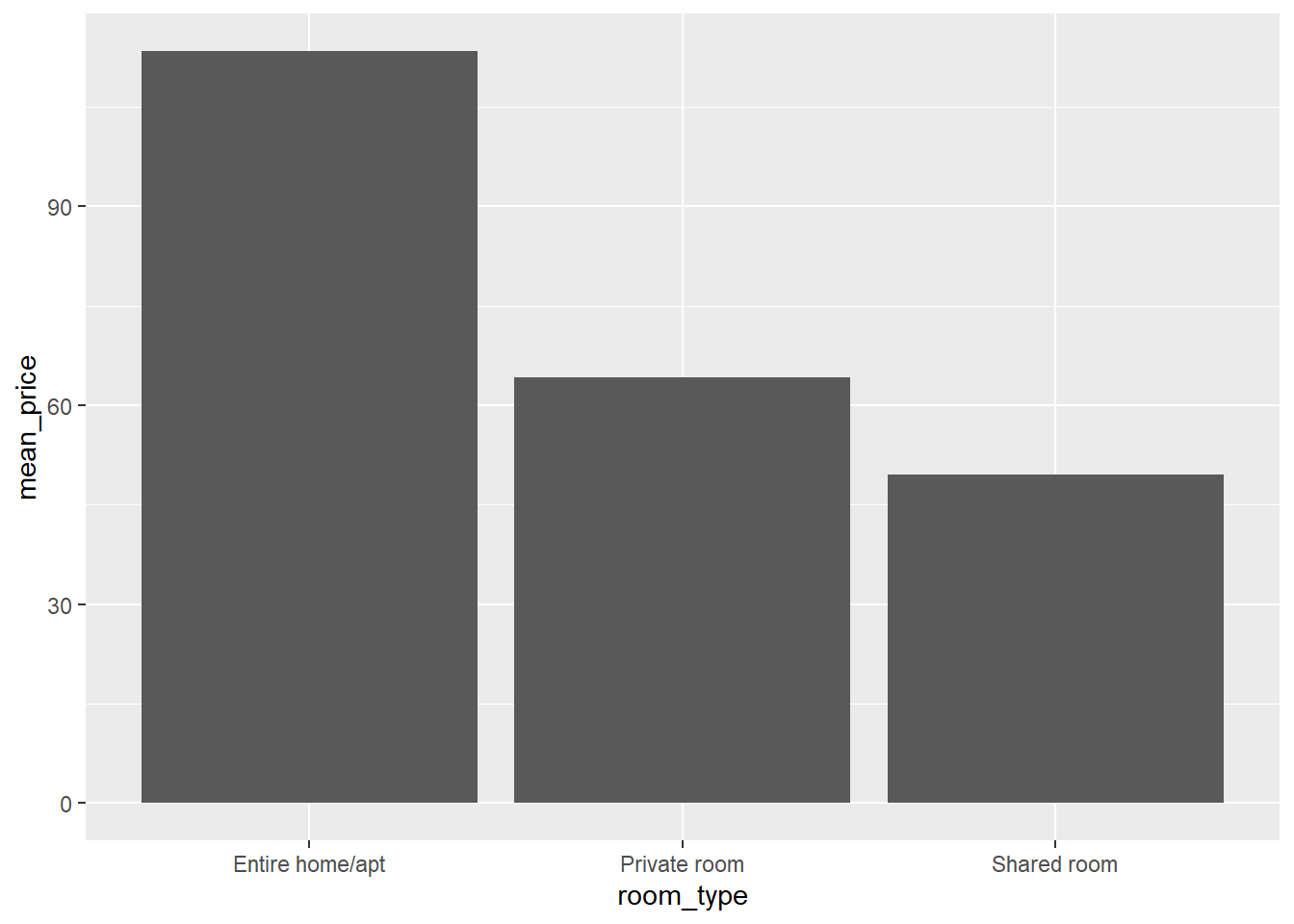
Unsurprisingly, entire homes or apartments are priced higher than private rooms, which in turn are priced higher than shared rooms. We also see that there are almost twice as many entire homes and apartments than private rooms available and there are hardly any shared rooms available. Also, the standard deviation is much higher in the entire homes or apartments category than in the private or shared room categories.
An ANOVA can test whether there are any significant differences in the mean prices per room type. But before we carry out an ANOVA, we need to check whether the assumptions for ANOVA are met.
3.3.1 Assumption: normality of residuals
The first assumption is that the dependent variable (price) is normally distributed at each level of the independent variable (room_type). First, let’s visually inspect whether this assumption will hold:
 # when creating a histogram, the dataset that serves as input to ggplot is the full dataset, not the summary with the means
ggplot(data = airbnb, mapping = aes(x = price)) + # We want price on the X-axis.
  facet_wrap(~ room_type) + # We want this split up per room_type. Facet_wrap will make sure ggplot creates different panels in your graph.
  geom_histogram() # geom_histogram makes sure the frequencies of the values on the X-axis are plotted.
## `stat_bin()` using `bins = 30`. Pick better value with `binwidth`.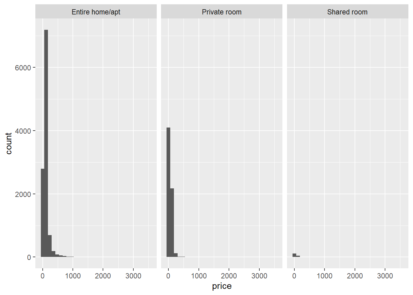
We see that there is right-skew for each room type. We can also formally test, within each room type, whether the distributions are normal with the Shapiro-Wilk test. For example, for the shared rooms:
airbnb.shared <- airbnb %>%
  filter(room_type == "Shared room") # retain data from only the shared rooms

shapiro.test(airbnb.shared$price)
##
## Shapiro-Wilk normality test
##
## data: airbnb.shared$price
## W = 0.83948, p-value = 1.181e-11The p-value of this test is extremely small, so the null hypothesis that the sample comes from a normal distribution should be rejected. If we try the Shapiro-Wilk test for the private rooms:
airbnb.private <- airbnb %>%
  filter(room_type == "Private room") # retain data from only the shared rooms

shapiro.test(airbnb.private$price)
## Error in shapiro.test(airbnb.private$price): sample size must be between 3 and 5000We get an error saying that our sample size is too large. To circumvent this problem, we can try the Anderson-Darling test from the nortest package:
install.packages("nortest")
library(nortest)ad.test(airbnb.private$price)##
## Anderson-Darling normality test
##
## data: airbnb.private$price
## A = 372.05, p-value < 2.2e-16Again, we reject the null hypothesis of normality. I leave it as an exercise to test the normality of the prices of the entire homes and apartments.
Now that we know the normality assumption is violated, what can we do? We can consider transforming our dependent variable with a log-transformation:
ggplot(data = airbnb, mapping = aes(x = log(price, base = exp(1)))) + # We want log-transformed price on the X-axis.
  facet_wrap(~ room_type) + # We want this split up per room_type. Facet_wrap will make sure ggplot creates different panels in your graph.
  geom_histogram() # geom_histogram makes sure the frequencies of the values on the X-axis are plotted.
## `stat_bin()` using `bins = 30`. Pick better value with `binwidth`.![]()
As you can see, a log-transformation normalizes a right-skewed distribution. We could then perform the ANOVA on the log-transformed dependent variable. However, in reality it is often safe to ignore violations of the normality assumption (unless you’re dealing with small samples, which we are not). We’re going to simply carry on with the untransformed price as dependent variable.
3.3.2 Assumption: homogeneity of variances
A second assumption we need to check is whether the variances of our dependent variable price are equal across the categories of our independent variable room_type. Normally, a box plot is informative:
ggplot(data = airbnb, mapping = aes(x = room_type, y = price)) +
  geom_boxplot()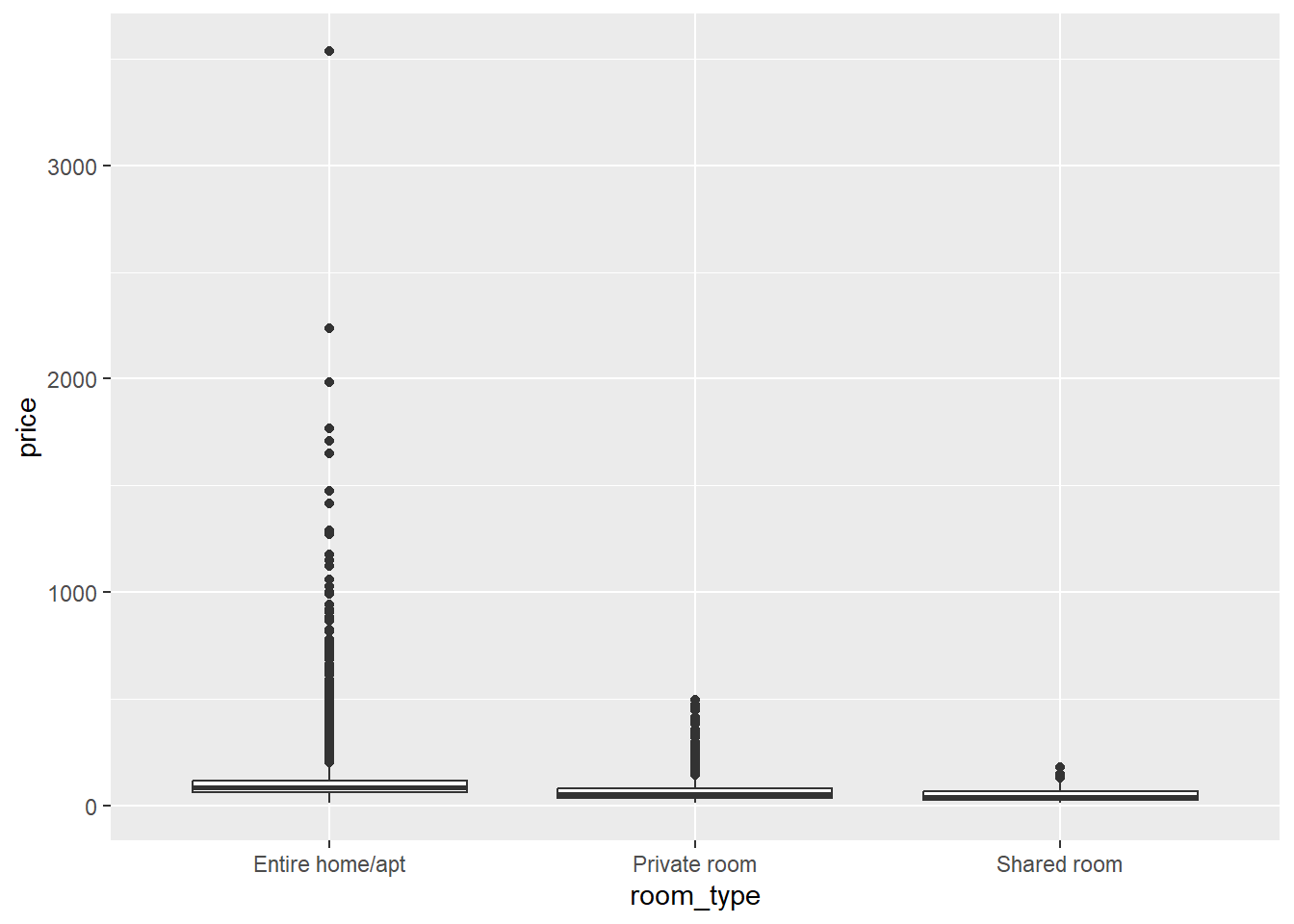
But in this case, the interquartile ranges (the heights of the boxes), which would normally give us an idea of the variance within each room type, are very narrow. This is because the range of Y-values to be plotted is very wide due to some extreme outliers. If we look at the standard deviations, however, we see that these are much higher for the entire rooms and apartments than for the private and shared rooms:
airbnb %>%
  group_by(room_type) %>%
  summarize(count = n(), # get the frequencies of the different room types
            mean_price = mean(price), # the average price per room type
            sd_price = sd(price)) # and the standard deviation of price per room type
## # A tibble: 3 × 4
## room_type count mean_price sd_price
## <chr> <int> <dbl> <dbl>
## 1 Entire home/apt 11082 113. 118.
## 2 Private room 6416 64.3 46.5
## 3 Shared room 153 49.6 33.9We can also carry out a formal test of homogeneity of variances. For this we need the function leveneTest from the package car:
install.packages("car") # For the test of equal variances, we need a package called car. We've installed this before, so no need to re-install it if you have done so already.
library(car)
# Levene's test of equal variances.
# Low p-value means the variances are not equal.
# First argument = continuous dependent variable, second argument = categorical independent variable.
leveneTest(airbnb$price, airbnb$room_type) ## Levene's Test for Homogeneity of Variance (center = median)
## Df F value Pr(>F)
## group 2 140.07 < 2.2e-16 ***
## 17648
## ---
## Signif. codes: 0 '***' 0.001 '**' 0.01 '*' 0.05 '.' 0.1 ' ' 1The p-value is extremely small, so we reject the null hypothesis of equal variances. As with the normality assumption, violations of the assumption of equal variances can, however, often be ignored and we will do so in this case.
3.3.3 The actual ANOVA
To carry out an ANOVA, we need to install some packages:
install.packages("remotes") # The remotes package allows us to install packages that are stored on GitHub, a website for package developers.
install.packages("car") # We'll need the car package as well to carry out the ANOVA (no need to re-install this if you have done this already).

library(remotes)
install_github('samuelfranssens/type3anova') # Install the type3anova package. This and the previous steps need to be carried out only once.

library(type3anova) # Load the type3anova package.
We can now proceed with the actual ANOVA:
# First create a linear model
# The lm() function takes a formula and a data argument
# The formula has the following syntax: dependent variable ~ independent variable(s)
linearmodel <- lm(price ~ room_type, data=airbnb)

# Then ask for output in ANOVA format. This gives Type III sum of squares.
# Note that this is different from anova(linearmodel) which gives Type I sum of squares.
type3anova(linearmodel)
## # A tibble: 3 × 6
## term ss df1 df2 f pvalue
## <chr> <dbl> <dbl> <int> <dbl> <dbl>
## 1 (Intercept) 7618725. 1 17648 803. 0
## 2 room_type 10120155. 2 17648 534. 0
## 3 Residuals 167364763. 17648 17648 NA NAIn this case the p-value associated with the effect of room_type is practically 0, which means that we reject the null hypothesis that the average price is equal for every room_type. You could report this as follows: “There were significant differences between the average prices of different room types (F(2, 17648) = 533.57, p < .001).”
3.3.4 Tukey’s honest significant difference test
Note that ANOVA tests the null hypothesis that the means in all our groups are equal. A rejection of this null hypothesis means that there is a significant difference in at least one of the possible pairs of means (i.e., in entire home/apartment vs. private and/or in entire home/apartment vs. shared and/or in private vs. shared). To get an idea of which pair of means contains a significant difference, we can follow up with Tukey’s test that will give us all pairwise comparisons. Tukey’s test corrects the p-values upwards — so it is more conservative in deciding something is significant — because the comparisons are post-hoc or exploratory:
TukeyHSD(aov(price ~ room_type, data=airbnb),
         "room_type") # The first argument is an "aov" object, the second is our independent variable.
## Tukey multiple comparisons of means
## 95% family-wise confidence level
##
## Fit: aov(formula = price ~ room_type, data = airbnb)
##
## $room_type
## diff lwr upr p adj
## Private room-Entire home/apt -49.11516 -52.69593 -45.534395 0.000000
## Shared room-Entire home/apt -63.79178 -82.37217 -45.211381 0.000000
## Shared room-Private room -14.67661 -33.34879 3.995562 0.155939This shows us that there’s no significant difference in the average price of shared and private rooms, but that shared rooms and private rooms both differ significantly from entire homes and apartments.
3.4 Linear regression
3.4.1 Simple linear regression
Say we want to predict price based on a number of room characteristics. Let’s start with a simple case where we predict price based on one predictor: overall satisfaction. Overall satisfaction is the rating that a listing gets on airbnb.com. Let’s make a scatterplot first:
ggplot(data = airbnb, mapping = aes(x = overall_satisfaction, y = price)) +
  geom_jitter() # jitter instead of points, otherwise many dots get drawn over each other
## Warning: Removed 7064 rows containing missing values (`geom_point()`).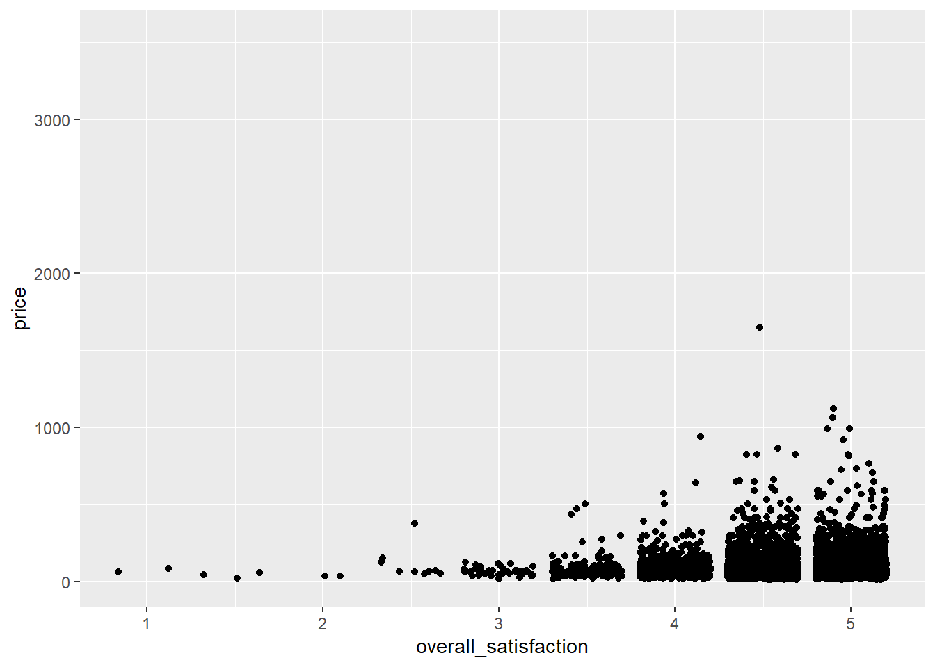
(We get an error message informing us that a number of rows were removed. These are the rows with missing values for overall_satisfaction, so there’s no need to worry about this error message. See data manipulations for why there are missing values for overall_satisfaction.)
The outliers on price reduce the informativeness of the graph, so let’s transform the price variable. Let’s also add some means to the graph, as we’ve learned here, and a regression line:
ggplot(data = airbnb, mapping = aes(x = overall_satisfaction, y = log(price, base = exp(1)))) +
  geom_jitter() + # jitter instead of points, otherwise many dots get drawn over each other
  stat_summary(fun.y=mean, colour="green", size = 4, geom="point", shape = 23, fill = "green") + # means
  stat_smooth(method = "lm", se=FALSE) # regression line
## `geom_smooth()` using formula = 'y ~ x'![]()
We see that price tends to increase slightly with increased satisfaction. To test whether the relationship between price and satisfaction is indeed significant, we can perform a simple regression (simple refers to the fact that there’s only one predictor):
linearmodel <- lm(price ~ overall_satisfaction, data = airbnb) # we create a linear model. The first argument is the model which takes the form of dependent variable ~ independent variable(s). The second argument is the data we should consider.

summary(linearmodel) # ask for a summary of this linear model
##
## Call:
## lm(formula = price ~ overall_satisfaction, data = airbnb)
##
## Residuals:
## Min 1Q Median 3Q Max
## -80.51 -38.33 -15.51 14.49 1564.67
##
## Coefficients:
## Estimate Std. Error t value Pr(>|t|)
## (Intercept) 29.747 8.706 3.417 0.000636 ***
## overall_satisfaction 12.353 1.864 6.626 3.62e-11 ***
## ---
## Signif. codes: 0 '***' 0.001 '**' 0.01 '*' 0.05 '.' 0.1 ' ' 1
##
## Residual standard error: 71.47 on 10585 degrees of freedom
## (7064 observations deleted due to missingness)
## Multiple R-squared: 0.00413, Adjusted R-squared: 0.004036
## F-statistic: 43.9 on 1 and 10585 DF, p-value: 3.619e-11We see two parameters in this model:
- \(\beta_0\) or the intercept (29.75)
- \(\beta_1\) or the slope of overall satisfaction (12.35)
These parameters have the following interpretations. The intercept (\(\beta_0\)) is the estimated price for an observation with overall_satisfaction equal to zero. The slope (\(\beta_1\)) is the estimated increase in price for every increase in overall satisfaction. This determines the steepness of the fitted regression line on the graph. So for a listing that has an overall satisfaction of, for example, 3.5, the estimated price is 29.75 + 3.5 \(\times\) 12.35 = 72.98.
The slope is positive and significant. You could report this as follows: “There was a significantly positive relationship between price and overall satisfaction (\(\beta\) = 12.35, t(10585) = 6.63, p < .001).”
In the output, we also get information about the overall model. The model comes with an F value of 43.9 with 1 degree of freedom in the numerator and 10585 degrees of freedom in the denominator. This F-statistic tells us whether our model with one predictor (overall_satisfaction) predicts the dependent variable (price) better than a model without predictors (which would simply predict the average of price for every level of overall satisfaction). The degrees of freedom allow us to find the corresponding p-value (< .001) of the F-statistic (43.9). The degrees of freedom in the numerator are equal to the number of predictors in our model. The degrees of freedom in the denominator are equal to the number of observations minus the number of predictors minus one. Remember that we have 10587 observations for which we have values for both price and overall_satisfaction. The p-value is smaller than .05, so we reject the null hypothesis that our model does not predict the dependent variable better than a model without predictors. Note that in the case of simple linear regression, the p-value of the model corresponds to the p-value of the single predictor. For models with more predictors, there is no such correspondence.
Finally, also note the R-squared statistic of the model. This statistic is equal to 0.004. This statistic tells us how much of the variance in the dependent variable is explained by our predictors. The more predictors you add to a model, the higher the R-squared will be.
3.4.2 Correlations
Note that in simple linear regression, the slope of the predictor is a function of the correlation between predictor and dependent variable. We can calculate the correlation as follows:
# Make sure to include the use argument, otherwise the result will be NA due to the missing values on overall_satisfaction.
# The use argument instructs R to calculate the correlation based only on the observations for which we have data on price and on overall_satisfaction.

cor(airbnb$price, airbnb$overall_satisfaction, use = "pairwise.complete.obs")
## [1] 0.06426892We see that the correlation is positive, but very low (\(r\) = 0.064).
Squaring this correlation will get you the R-squared of a model with only that predictor (0.064 \(\times\) 0.064 = 0.004).
When dealing with multiple predictors (as in the next section), we may want to generate a correlation matrix. This is especially useful when checking for multicollinearity. Say we want the correlations between, price, overall_satisfaction, reviews, accommodates:
airbnb.corr <- airbnb %>%
  filter(!is.na(overall_satisfaction)) %>% # otherwise you'll see NA's in the result
  select(price, overall_satisfaction, reviews, accommodates)

cor(airbnb.corr) # get the correlation matrix
## price overall_satisfaction reviews accommodates
## price 1.00000000 0.06426892 -0.05827489 0.63409855
## overall_satisfaction 0.06426892 1.00000000 0.03229339 -0.04698709
## reviews -0.05827489 0.03229339 1.00000000 -0.03862767
## accommodates 0.63409855 -0.04698709 -0.03862767 1.00000000You can easily visualize this correlation matrix:
install.packages("corrplot") # install and load the corrplot package
library(corrplot)corrplot(cor(airbnb.corr), method = "number", type = "lower", bg = "grey") # put this in a nice table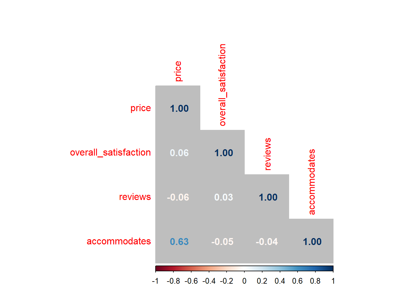
The colors of the correlations depend on their absolute values.
You can also get p-values for the correlations (p < .05 tells you the correlation differs significantly from zero):
# The command for the p-values is cor.mtest(airbnb.corr)
# But we want only the p-values, hence $p
# And we round them to five digits, hence round( , 5)

round(cor.mtest(airbnb.corr)$p, 5)
## price overall_satisfaction reviews accommodates
## price 0 0.00000 0.00000 0e+00
## overall_satisfaction 0 0.00000 0.00089 0e+00
## reviews 0 0.00089 0.00000 7e-05
## accommodates 0 0.00000 0.00007 0e+003.4.3 Multiple linear regression, without interaction
Often, we want to use more than one continuous independent variable to predict the continuous dependent variable. For example, we may want to use overall satisfaction and the number of reviews to predict the price of an Airbnb listing. The number of reviews can be seen as an indicator of how many people have stayed at a listing before. We can include both predictors (overall_satisfaction & reviews) in a model:
linearmodel <- lm(price ~ overall_satisfaction + reviews, data = airbnb)
summary(linearmodel)
##
## Call:
## lm(formula = price ~ overall_satisfaction + reviews, data = airbnb)
##
## Residuals:
## Min 1Q Median 3Q Max
## -83.18 -36.97 -16.07 13.80 1562.08
##
## Coefficients:
## Estimate Std. Error t value Pr(>|t|)
## (Intercept) 30.95504 8.69242 3.561 0.000371 ***
## overall_satisfaction 12.72777 1.86196 6.836 8.61e-12 ***
## reviews -0.10370 0.01663 -6.236 4.65e-10 ***
## ---
## Signif. codes: 0 '***' 0.001 '**' 0.01 '*' 0.05 '.' 0.1 ' ' 1
##
## Residual standard error: 71.35 on 10584 degrees of freedom
## (7064 observations deleted due to missingness)
## Multiple R-squared: 0.007776, Adjusted R-squared: 0.007589
## F-statistic: 41.48 on 2 and 10584 DF, p-value: < 2.2e-16With this model, estimated price = \(\beta_0\) + \(\beta_1\) \(\times\) overall_satisfaction + \(\beta_2\) \(\times\) reviews, where:
- \(\beta_0\) is the intercept (30.96)
- \(\beta_1\) represents the relationship between overall satisfaction and price (12.73), controlling for all other variables in our model
- \(\beta_2\) represents the relationship between reviews and price (-0.1), controlling for all other variables in our model
For a given level of reviews, the relationship between overall_satisfaction and price can be re-written as:
= [\(\beta_0\) + \(\beta_2\) \(\times\)reviews] + \(\beta_1\) \(\times\) overall_satisfaction
We see that only the intercept (\(\beta_0\) + \(\beta_2\) \(\times\)reviews) but not the slope (\(\beta_1\)) of the relationship between overall satisfaction and price depends on the number of reviews. This will change when we add an interaction between reviews and overall satisfaction (see next section).
Similarly, for a given level of overall_satisfaction, the relationship between reviews and price can be re-written as:
= [\(\beta_0\) + \(\beta_1\) \(\times\) overall_satisfaction] + \(\beta_2\) \(\times\) reviews
3.4.4 Multiple linear regression, with interaction
Often, we’re interested in interactions between predictors (e.g., overall_satisfaction & reviews). An interaction between predictors tells us that the effect of one predictor depends on the level of the other predictor:
# overall_satisfaction + reviews: the interaction is not included as a predictor
# overall_satisfaction * reviews: the interaction between the two predictors is included as a predictor

linearmodel <- lm(price ~ overall_satisfaction * reviews, data = airbnb)
summary(linearmodel)
##
## Call:
## lm(formula = price ~ overall_satisfaction * reviews, data = airbnb)
##
## Residuals:
## Min 1Q Median 3Q Max
## -82.17 -36.71 -16.08 13.47 1561.53
##
## Coefficients:
## Estimate Std. Error t value Pr(>|t|)
## (Intercept) 48.77336 10.14434 4.808 1.55e-06 ***
## overall_satisfaction 8.91437 2.17246 4.103 4.10e-05 ***
## reviews -0.99200 0.26160 -3.792 0.00015 ***
## overall_satisfaction:reviews 0.18961 0.05573 3.402 0.00067 ***
## ---
## Signif. codes: 0 '***' 0.001 '**' 0.01 '*' 0.05 '.' 0.1 ' ' 1
##
## Residual standard error: 71.31 on 10583 degrees of freedom
## (7064 observations deleted due to missingness)
## Multiple R-squared: 0.008861, Adjusted R-squared: 0.00858
## F-statistic: 31.54 on 3 and 10583 DF, p-value: < 2.2e-16With this model, estimated price = \(\beta_0\) + \(\beta_1\) \(\times\) overall_satisfaction + \(\beta_2\) \(\times\) reviews + \(\beta_3\) \(\times\) overall_satisfaction \(\times\) reviews, where:
- \(\beta_0\) is the intercept (48.77)
- \(\beta_1\) represents the relationship between overall satisfaction and price (8.91), controlling for all other variables in our model
- \(\beta_2\) represents the relationship between reviews and price (-0.99), controlling for all other variables in our model
- \(\beta_3\) is the interaction between overall satisfaction and reviews (0.19)
For a given level of reviews, the relationship between overall_satisfaction and price can be re-written as:
= [\(\beta_0\) + \(\beta_2\) \(\times\)reviews] + (\(\beta_1\) + \(\beta_3\) \(\times\) reviews) \(\times\) overall_satisfaction
We see that both the intercept (\(\beta_0\) + \(\beta_2\) \(\times\)reviews) and the slope (\(\beta_1\) + \(\beta_3\) \(\times\) reviews) of the relationship between overall satisfaction and price depend on the number of reviews. In the model without interactions, only the intercept of the relationship between overall satisfaction and price depended on the number of reviews. Because we’ve added an interaction between overall satisfaction and number of reviews to our model, the slope now also depends on the number of reviews.
Similarly, for a given level of overall_satisfaction, the relationship between reviews and price can be re-written as:
= [\(\beta_0\) + \(\beta_1\) \(\times\) overall_satisfaction] + (\(\beta_2\) + \(\beta_3\) \(\times\) overall_satisfaction) \(\times\) reviews
Here as well, we see that both the intercept and the slope of the relationship between reviews and price depend on the overall satisfaction.
As said, when the relationship between an independent variable and a dependent variable depends on the level of another independent variable, then we have an interaction between the two independent variables. For these data, the interaction is highly significant (p < .001). Let’s visualize this interaction. We focus on the relationship between overall satisfaction and price. We’ll plot this for a level of reviews that can be considered low, medium, and high:
airbnb %>%
  filter(!is.na(overall_satisfaction)) %>%
  summarize(min = min(reviews),
            Q1 = quantile(reviews, .25), # first quartile
            Q2 = quantile(reviews, .50), # second quartile or median
            Q3 = quantile(reviews, .75), # third quartile
            max = max(reviews),
            mean = mean(reviews))
## # A tibble: 1 × 6
## min Q1 Q2 Q3 max mean
## <dbl> <dbl> <dbl> <dbl> <dbl> <dbl>
## 1 3 6 13 32 708 28.5We see that 25% of listings has 6 or less reviews, 50% of listings has 13 or less reviews, and 75% of listings has 32 or less reviews.
We want three groups, however, so we could ask for different quantiles:
airbnb %>%
  filter(!is.na(overall_satisfaction)) %>%
  summarize(Q1 = quantile(reviews, .33), # low
            Q2 = quantile(reviews, .66), # medium
            max = max(reviews))          # high
## # A tibble: 1 × 3
## Q1 Q2 max
## <dbl> <dbl> <dbl>
## 1 8 23 708and make groups based on these numbers:
airbnb.reviews <- airbnb %>%
  filter(!is.na(overall_satisfaction)) %>%
  mutate(review_group = case_when(reviews <= quantile(reviews, .33) ~ "low",
                                  reviews <= quantile(reviews, .66) ~ "medium",
                                  TRUE                              ~ "high"),
         review_group = factor(review_group, levels = c("low","medium","high")))
So we tell R to make a new variable review_group that should be equal to "low" when the number of reviews is less than or equal to the 33rd percentile, "medium" when the number of reviews is less than or equal to the 66th percentile, and "high" otherwise. Afterwards, we factorize the newly created review_group variable and provide a new argument, levels, that specifies the order of the factor levels (otherwise the order would be alphabetical: high, low, medium). Let’s check whether the grouping was successful:
# check:
airbnb.reviews %>%
  group_by(review_group) %>%
  summarize(min = min(reviews), max = max(reviews))
## # A tibble: 3 × 3
## review_group min max
## <fct> <dbl> <dbl>
## 1 low 3 8
## 2 medium 9 23
## 3 high 24 708Indeed, the maximum numbers of reviews in each group correspond to the cut-off points set above. We can now ask R for a graph of the relationship between overall satisfaction and price for the three levels of review:
ggplot(data = airbnb.reviews, mapping = aes(x = overall_satisfaction, y = log(price, base = exp(1)))) + # log transform price
  facet_wrap(~ review_group) + # ask for different panels for each review group
  geom_jitter() +
  stat_smooth(method = "lm", se = FALSE)
## `geom_smooth()` using formula = 'y ~ x'
We see that the relationship between overall satisfaction and price is always positive, but it is more positive for listings with many reviews than for listings with few reviews. There could be many reasons for this. Perhaps it is the case that listings with positive reviews increase their price, but only after they’ve received a certain amount of reviews.
We also see that listings with many reviews hardly ever have a satisfaction rating less than 3. This makes sense, because it is hard to keep attracting people when a listing’s rating is low. Listings with few reviews do tend to have low overall satisfaction ratings. So it seems that our predictors are correlated: the more reviews a listing has, the higher its satisfaction rating will be. This potentially presents a problem that we’ll discuss in one of the next sections on multicollinearity.
3.4.5 Assumptions
Before drawing conclusions from a regression analysis, one has to check a number of assumptions. These assumptions should be met regardless of the number of predictors in the model, but we’ll continue with the case of two predictors.
3.4.5.1 Normality of residuals
The residuals (the difference between observed and estimated values) should be normally distributed. We can visually inspect the residuals:
linearmodel <- lm(price ~ overall_satisfaction * reviews, data = airbnb)
residuals <- as_tibble(resid(linearmodel))
# ask for the residuals of the linear model with resid(linearmodel)
# and turn this in a data frame with as_tibble()

ggplot(data = residuals, mapping = aes(x = value)) +
  geom_histogram()
## `stat_bin()` using `bins = 30`. Pick better value with `binwidth`.
3.4.5.2 Homoscedasticity of residuals
The residuals (the difference between observed and estimated values) should have a constant variance. We can check this by plotting the residuals versus the predicted values:
linearmodel <- lm(price ~ overall_satisfaction * reviews, data = airbnb)

 # create a data frame (a tibble)
residuals_predicted <- tibble(residuals = resid(linearmodel), # the first variable is residuals which are the residuals of our linear model
                              predicted = predict(linearmodel)) # the second variable is predicted which are the predicted values of our linear model

ggplot(data = residuals_predicted, mapping = aes(x = predicted, y = residuals)) +
  geom_point()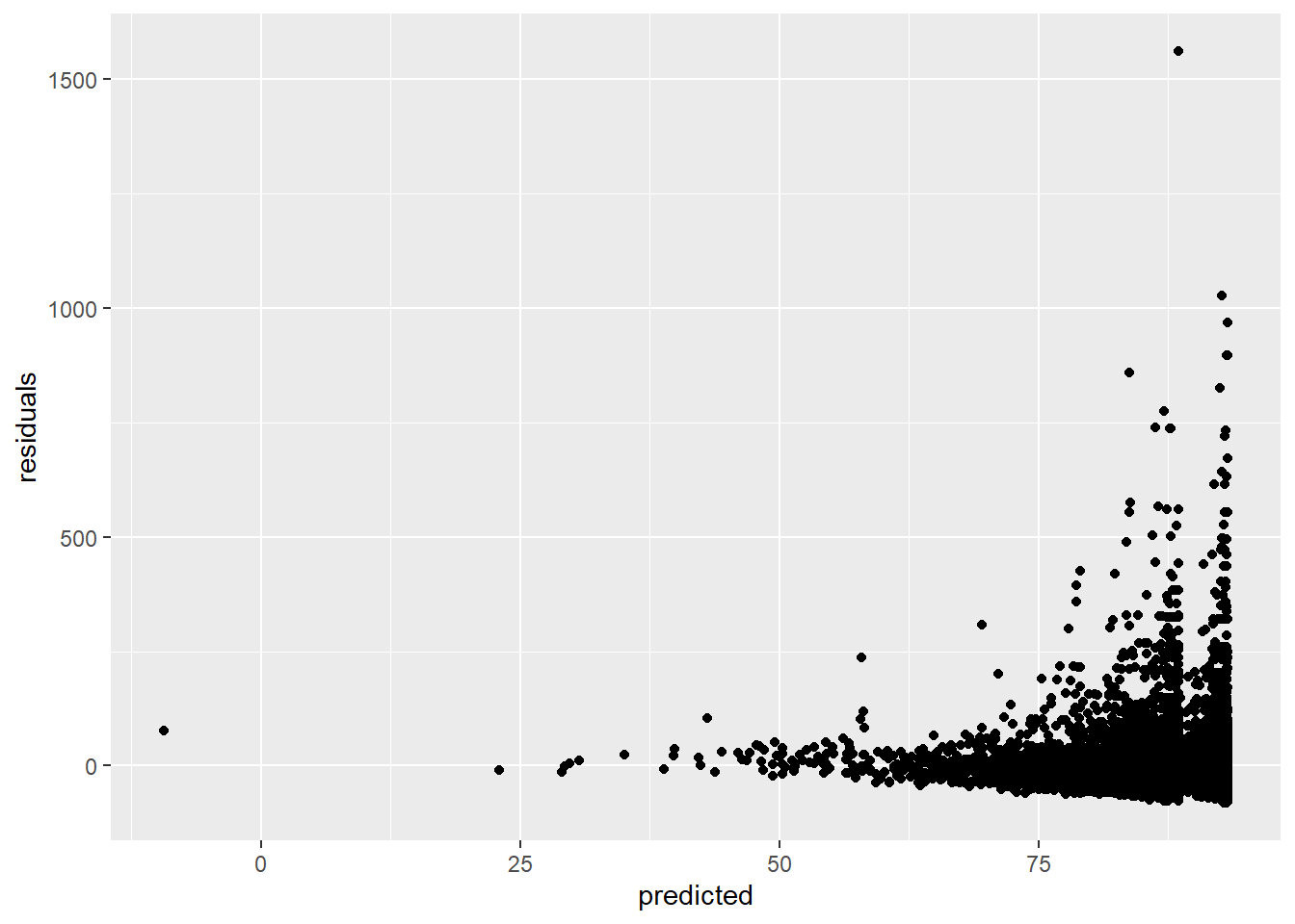
This assumption is violated, because the larger our predicted values become, the more variance we see in the residuals.
3.4.5.3 Multicollinearity
Multicollinearity exists whenever two or more of the predictors in a regression model are moderately or highly correlated (so this of course is not a problem in the case of simple regression). Let’s test the correlation between overall satisfaction and number of reviews:
# Make sure to include the use argument, otherwise the result will be NA due to the missing values on overall_satisfaction.
# The use argument instructs R to calculate the correlation based only on the observations for which we have data on price and on overall_satisfaction.

cor.test(airbnb$overall_satisfaction,airbnb$reviews, use = "pairwise.complete.obs") # test for correlation
##
## Pearson's product-moment correlation
##
## data: airbnb$overall_satisfaction and airbnb$reviews
## t = 3.3242, df = 10585, p-value = 0.0008898
## alternative hypothesis: true correlation is not equal to 0
## 95 percent confidence interval:
## 0.01325261 0.05131076
## sample estimates:
## cor
## 0.03229339Our predictors are indeed significantly correlated (p < .001), but the correlation is really low (0.03). When dealing with more than two predictors, it’s a good idea to make a correlation matrix.
The problem with multicollinearity is that it inflates the standard errors of the regression coefficients. As a result, the significance tests of these coefficients will find it harder to reject the null hypothesis. We can easily get an idea of the degree to which coefficients are inflated. To illustrate this, let’s estimate a model with predictors that are correlated: accommodates and price (\(r\) = 0.56)
linearmodel <- lm(overall_satisfaction ~  accommodates * price, data = airbnb)
summary(linearmodel)
##
## Call:
## lm(formula = overall_satisfaction ~ accommodates * price, data = airbnb)
##
## Residuals:
## Min 1Q Median 3Q Max
## -3.6494 -0.1624 -0.1105 0.3363 0.6022
##
## Coefficients:
## Estimate Std. Error t value Pr(>|t|)
## (Intercept) 4.622e+00 9.938e-03 465.031 < 2e-16 ***
## accommodates -1.640e-02 2.039e-03 -8.046 9.48e-16 ***
## price 1.356e-03 1.159e-04 11.702 < 2e-16 ***
## accommodates:price -5.423e-05 9.694e-06 -5.595 2.26e-08 ***
## ---
## Signif. codes: 0 '***' 0.001 '**' 0.01 '*' 0.05 '.' 0.1 ' ' 1
##
## Residual standard error: 0.3689 on 10583 degrees of freedom
## (7064 observations deleted due to missingness)
## Multiple R-squared: 0.0199, Adjusted R-squared: 0.01963
## F-statistic: 71.64 on 3 and 10583 DF, p-value: < 2.2e-16We see that all predictors are significant. Let’s have a look at the variance inflation factors:
library(car) # the vif function is part of the car package

vif(linearmodel)
## there are higher-order terms (interactions) in this model
## consider setting type = 'predictor'; see ?vif## accommodates price accommodates:price
## 2.090206 5.359203 6.678312The VIF factors tells you the degree to which the standard errors are inflated. A rule of thumb is that VIF’s of 5 and above indicate significant inflation.
3.5 Chi-squared test
Suppose we’re interested in finding a true gem of a listing. For example, we’re interested in listings with a 5 out of 5 rating and at least 30 reviews:
airbnb <- airbnb %>%
  mutate(gem = (overall_satisfaction == 5 & reviews>=30), # two conditions should be met before saying a listing is a gem
         gem = factor(gem, labels = c("no gem","gem")))  # give the logical variable more intuitive labels
Now, say we’re interested in knowing whether we’re more likely to find gems in small or in large cities (we’ve created the size variable here). The chi-squared test can provide an answer to this question by testing the null hypothesis of no relationship between two categorical variables (city size: large vs. small & gem: yes vs. no). It compares the observed frequency table with the frequency table that you would expect when there is no relation between the two variables. The more the observed and the expected frequency tables diverge, the larger the chi-squared statistic, the lower the p-value, and the less likely it is that the two variables are unrelated.
Before we carry out a chi-squared test, remember that some cities have a missing value for size because they have a missing value for population. Let’s filter these out first:
airbnb.cities <- airbnb %>%
  filter(!is.na(size))

# we only want those observations where size is not NA. ! stands for 'not'
# check out https://r4ds.had.co.nz/transform.html#filter-rows-with-filter for more logical operators (scroll down to section 5.2.2)
Now, print the frequencies of the city size and gem combinations:
airbnb.cities %>%
  group_by(size, gem) %>%
  summarize(count = n())
## `summarise()` has grouped output by 'size'. You can override using the `.groups` argument.## # A tibble: 4 × 3
## # Groups: size [2]
## size gem count
## <fct> <fct> <int>
## 1 small no gem 4095
## 2 small gem 175
## 3 large no gem 10117
## 4 large gem 912This information is correct but the format in which the table is presented is a bit unusual. We would like to have one variable as rows and the other as columns:
table(airbnb.cities$size, airbnb.cities$gem)##
## no gem gem
## small 4095 175
## large 10117 912This is a bit easier to interpret. A table like this is often called a cross table. It’s quite to easy to ask for percentages instead of counts:
crosstable <- table(airbnb.cities$size, airbnb.cities$gem) # We need to save the cross table first.
prop.table(crosstable) # Use the prop.table() function to ask for percentages.
##
## no gem gem
## small 0.26766455 0.01143866
## large 0.66128505 0.05961174prop.table(crosstable,1) # This gives percentages conditional on rows, i.e., the percentages in the rows sum to 1.##
## no gem gem
## small 0.95901639 0.04098361
## large 0.91730891 0.08269109prop.table(crosstable,2) # This gives percentages conditional on columns, i.e., the percentages in the columns sum to 1.##
## no gem gem
## small 0.2881368 0.1609936
## large 0.7118632 0.8390064Based on these frequencies or percentages, we should not expect a strong relation between size and gem. Let’s carry out the chi-squared test to test our intuition:
chisq.test(crosstable)##
## Pearson's Chi-squared test with Yates' continuity correction
##
## data: crosstable
## X-squared = 80.497, df = 1, p-value < 2.2e-16The value of the chi statistic is 80.5 and the p-value is practically 0, so we reject the null hypothesis of no relationship. This is not what we expected, but the p-value is this low because our sample is quite large (15299 observations). You could report this as follows: “There was a significant relationship between city size and whether or not a listing was a gem (\(\chi^2\)(1, N = 15299) = 80.5, p < .001), such that large cities (8.27%) had a higher percentage of gems than small cities (4.1%).”
3.6 Logistic regression (optional)
Sometimes we want to predict a binary dependent variable, i.e., a variable that can only take on two values, based on a number of continuous or categorical independent variables. For example, say we’re interested in testing whether or not a listing is a gem depends on the price and the room type of the listing.
We cannot use ANOVA or linear regression here because the dependent variable is a binary variable and hence not normally distributed. Another problem with ANOVA or linear regression, is that it may predict values that are not possible (e.g., our predicted value may be 5, but only 0 and 1 make sense for this dependent variable). Therefore, we will use logistic regression. Logistic regression first transforms the dependent variable \(\textrm{Y}\) with the logit transformation. The logit transformation takes the natural logarithm of the odds that the dependent variable is equal to 1:
\(\textrm{odds} = \dfrac{P(Y = 1)}{P(Y = 0)} = \dfrac{P(Y = 1)}{1 - P(Y = 1)}\)
and then \(\textrm{logit}(P(Y = 1)) = \textrm{ln}(\dfrac{P(Y = 1)}{1 - P(Y = 1)})\).
This makes sure our dependent variable is normally distributed and is not constrained to be either 0 or 1.
Let’s carry out the logistic regression:
logistic.model <- glm(gem ~ price * room_type, data=airbnb, family="binomial") # the family = "binomial" argument tells R to treat the dependent variable as a 0 / 1 variable
summary(logistic.model) # ask for the regression output
##
## Call:
## glm(formula = gem ~ price * room_type, family = "binomial", data = airbnb)
##
## Deviance Residuals:
## Min 1Q Median 3Q Max
## -0.4909 -0.3819 -0.3756 -0.3660 2.5307
##
## Coefficients:
## Estimate Std. Error z value Pr(>|z|)
## (Intercept) -2.5270702 0.0570207 -44.318 <2e-16 ***
## price -0.0007185 0.0004030 -1.783 0.0746 .
## room_typePrivate room -0.0334362 0.1072091 -0.312 0.7551
## room_typeShared room 1.0986318 1.1278159 0.974 0.3300
## price:room_typePrivate room -0.0011336 0.0012941 -0.876 0.3810
## price:room_typeShared room -0.0562610 0.0381846 -1.473 0.1406
## ---
## Signif. codes: 0 '***' 0.001 '**' 0.01 '*' 0.05 '.' 0.1 ' ' 1
##
## (Dispersion parameter for binomial family taken to be 1)
##
## Null deviance: 8663.8 on 17650 degrees of freedom
## Residual deviance: 8648.6 on 17645 degrees of freedom
## AIC: 8660.6
##
## Number of Fisher Scoring iterations: 7We see that the only marginally significant predictor of whether or not a listing is a gem, is the price of the listing. You could report this as follows: “Controlling for room type and the interaction between price and room type, there was a marginally significant negative relationship between price and the probability of a listing being a gem (\(\beta\) = -0.0007185, \(\chi\)(17645) = -1.783, p = 0.075).”
The interpretation of the regression coefficients in logistic regression is different than in the case of linear regression:
summary(logistic.model)##
## Call:
## glm(formula = gem ~ price * room_type, family = "binomial", data = airbnb)
##
## Deviance Residuals:
## Min 1Q Median 3Q Max
## -0.4909 -0.3819 -0.3756 -0.3660 2.5307
##
## Coefficients:
## Estimate Std. Error z value Pr(>|z|)
## (Intercept) -2.5270702 0.0570207 -44.318 <2e-16 ***
## price -0.0007185 0.0004030 -1.783 0.0746 .
## room_typePrivate room -0.0334362 0.1072091 -0.312 0.7551
## room_typeShared room 1.0986318 1.1278159 0.974 0.3300
## price:room_typePrivate room -0.0011336 0.0012941 -0.876 0.3810
## price:room_typeShared room -0.0562610 0.0381846 -1.473 0.1406
## ---
## Signif. codes: 0 '***' 0.001 '**' 0.01 '*' 0.05 '.' 0.1 ' ' 1
##
## (Dispersion parameter for binomial family taken to be 1)
##
## Null deviance: 8663.8 on 17650 degrees of freedom
## Residual deviance: 8648.6 on 17645 degrees of freedom
## AIC: 8660.6
##
## Number of Fisher Scoring iterations: 7The regression coefficient of price is -0.0007185. This means that a one unit increase in price will lead to a -0.0007185 increase in the log odds of gem being equal to 1 (i.e., of a listing being a gem). For example:
\(\textrm{logit}(P(Y = 1 | \textrm{price} = 60 )) = \textrm{logit}(P(Y = 1 | \textrm{price} = 59 )) - 0.0007185\)
\(\Leftrightarrow \textrm{logit}(P(Y = 1 | \textrm{price} = 60 )) - \textrm{logit}(P(Y = 1 | \textrm{price} = 59 )) = -0.0007185\)
\(\Leftrightarrow \textrm{ln(odds}(P(Y = 1 | \textrm{price} = 60 )) - \textrm{ln(odds}(P(Y = 1 | \textrm{price} = 59 )) = -0.0007185\)
\(\Leftrightarrow \textrm{ln}(\dfrac{ \textrm{odds}(P(Y = 1 | \textrm{price} = 60 )}{\textrm{odds}(P(Y = 1 | \textrm{price} = 59 )}) = -0.0007185\)
\(\Leftrightarrow \dfrac{ \textrm{odds}(P(Y = 1 | \textrm{price} = 60 )}{\textrm{odds}(P(Y = 1 | \textrm{price} = 59 )} = e^{-0.0007185}\)
\(\Leftrightarrow \textrm{odds}(P(Y = 1 | \textrm{price} = 60 ) = e^{-0.0007185} * \textrm{odds}(P(Y = 1 | \textrm{price} = 59 )\)
Thus the regression coefficient in a logistic regression should be interpreted as the relative increase in the odds of the dependent variable being equal to 1, for every unit increase in the predictor, controlling for all other factors in our model. In this case, the odds of a listing being a gem should be multiplied by \(e^{-0.0007185}\) = 0.999 or should be decreased with 0.1 percent, for every one unit increase in price. In other words, more expensive listings are less likely to be gems. In the specific example above, the odds of being a gem of a listing priced 60 is \(e^{(-0.0007185 \times 5)}\) = 0.996 times the odds of being a gem of a listing priced 59.
3.6.1 Measuring the fit of a logistic regression: percentage correctly classified
Our model uses the listing’s price and room type to predict whether the listing is a gem or not. When making predictions, it’s natural to ask ourselves whether our predictions are any good. In other words, using price and room type, how often do we correctly predict whether a listing is a gem or not? To get an idea of the quality of our predictions, we can take the price and the room type of the listings in our dataset, predict whether the listings are gems, and compare our predictions to the actual gem status of the listings. Let’s first make the predictions:
airbnb <- airbnb %>%
  mutate(prediction = predict(logistic.model, airbnb))
# Create a new column called prediction in the airbnb data frame and store in that the prediction,
# based on logistic.model, for the airbnb data

# Have a look at those predictions:
head(airbnb$prediction)
## 1 2 3 4 5 6
## -4.790232 -4.448355 -4.049498 -4.619293 -4.106477 -4.847211# Compare it with the observations:
head(airbnb$gem)## [1] no gem no gem no gem no gem no gem no gem
## Levels: no gem gemDo you see the problem? The predictions are logits, i.e., logarithms of odds that the listings are gems, but the observations simply tell us whether a listing is a gem or not. For a meaningful comparison between predictions and observations, we need to transform the logits into a decision: gem or no gem. It’s easy to transform logits into odds by taking the exponential of the logit. The relationship between odds and probabilities is the following:
\(\textrm{odds} = \dfrac{P(Y = 1)}{P(Y = 0)} = \dfrac{P(Y = 1)}{1 - P(Y = 1)}\)
\(\Leftrightarrow \dfrac{odds}{1 + \dfrac{P(Y = 1)}{1 - P(Y = 1)}} = \dfrac{\dfrac{P(Y = 1)}{1 - P(Y = 1)}}{1 + \dfrac{P(Y = 1)}{1 - P(Y = 1)}}\)
\(\Leftrightarrow \dfrac{odds}{1 + odds} = \dfrac{\dfrac{P(Y = 1)}{1 - P(Y = 1)}}{\dfrac{1 - P(Y = 1) + P(Y = 1)}{1 - P(Y = 1)}}\)
\(\Leftrightarrow \dfrac{odds}{1 + odds} = \dfrac{P(Y = 1)}{1 - P(Y = 1) + P(Y = 1)}\)
\(\Leftrightarrow \dfrac{odds}{1 + odds} = P(Y = 1)\)
Now let’s calculate, for each listing, the probability that the listing is a gem:
airbnb <- airbnb %>%
  mutate(prediction.logit = predict(logistic.model, airbnb),
         prediction.odds = exp(prediction.logit),
         prediction.probability = prediction.odds / (1+prediction.odds))

# Have a look at the predicted probabilities:
head(airbnb$prediction.probability)
## 1 2 3 4 5 6
## 0.008242034 0.011562542 0.017132489 0.009763496 0.016198950 0.007789092The first few numbers are very low probabilities, but there are some higher probabilities as well and all predictions lie between 0 and 1, as they should. We now need to decide which probability is enough for us to predict that a listing is a gem or not. An obvious choice is a probability of 0.5: A probability higher than 0.5 means we predict it’s more likely that a listing is gem than that it is not. Let’s convert probabilities into predictions:
airbnb <- airbnb %>%
  mutate(prediction = case_when(prediction.probability<=.50 ~ "no gem",
                                prediction.probability> .50 ~ "gem"))

# Have a look at the predictions:
head(airbnb$prediction)
## [1] "no gem" "no gem" "no gem" "no gem" "no gem" "no gem"A final step is to compare predictions with observations:
table(airbnb$prediction, airbnb$gem)##
## no gem gem
## no gem 16471 1180Normally, we’d see a 2x2 table, but we see a table with one predicted value in the rows and two observed values in the columns. This is because all predicted probabilities are below .50 and therefore we always predict no gem. Let’s lower the treshold to predict that a listing is a gem:
airbnb <- airbnb %>%
  mutate(prediction = case_when(prediction.probability<=.07 ~ "no gem",
                                prediction.probability> .07 ~ "gem"),
         prediction = factor(prediction, levels = c("no gem","gem"))) # make sure no gem is the first level of our factor

# Have a look at the table:
table(airbnb$prediction,airbnb$gem)
##
## no gem gem
## no gem 11240 854
## gem 5231 326We can see that with this decision rule (predict gem whenever the predicted probability of gem is higher than 7%), we get 11240 + 326 predictions correct and 5231 + 854 predictions wrong, which is a hit rate of (11240 + 326) / (11240 + 326 + 5231 + 854) = 65.5%.