6 Principal component analysis for perceptual maps (toothpaste dataset)
In this chapter, you will learn how to carry out a principal component analysis and visualize the results in a perceptual map.
Say we have a set of observations that differ from each other on a number of dimensions, for example, we have a number of whiskey brands (observations) that are rated on a number of attributes such as body, sweetness, fruitiness, etc (dimensions). If some of those dimensions are strongly correlated then it should be possible to describe the observations by a smaller (than original) number of dimensions without losing too much information. For example, sweetness and fruitness could be highly correlated and could therefore be replaced by one variable. Such dimensionality reduction is the goal of principal component analysis.
6.1 Data
6.1.1 Import
We will analyze data from a survey in which 60 consumers were asked to respond to six questions about toothpaste. These data were collected by the creators of Radiant, which is an R package for business analytics that we will use later on. Download the data here and import them into R:
library(tidyverse)
library(readxl)

toothpaste <- read_excel("toothpaste.xlsx")
6.1.2 Manipulate
toothpaste # Check out the dataThe data set consists of one identifier, consumer, and the respondent’s ratings of the importance of six toothpaste attributes: prevents_cavities, shiny_teeth, strengthens_gums, freshens_breath, decay_prevention_unimportant, and attractive_teeth. We also have the respondent’s age and gender.
Let’s factorize the identifier and gender:
toothpaste <- toothpaste %>%
  mutate(consumer = factor(consumer),
         gender = factor(gender))
6.1.3 Recap: importing & manipulating
Here’s what we’ve done so far, in one orderly sequence of piped operations (download the data here):
library(tidyverse)
library(readxl)

toothpaste <- read_excel("toothpaste.xlsx")
  mutate(consumer = factor(consumer),
         gender = factor(gender))
6.2 How many factors should we retain?
The goal of principal component analysis is to reduce the number of dimensions that describe our data, without losing too much information. The first step in principal component analysis is to decide upon the number of principal components or factors we want to retain. To help us decide, we’ll use the pre_factor function from the radiant package:
install.packages("radiant")
library(radiant)
# store the names of the dimensions in a vector so that we don't have to type them again and again
dimensions <- c("prevents_cavities", "shiny_teeth", "strengthens_gums", "freshens_breath", "decay_prevention_unimportant", "attractive_teeth")
# hint: we could also do this as follows:
# dimensions <- toothpaste %>% select(-consumer, -gender, -age) %>% names()
summary(pre_factor(toothpaste, vars = dimensions))## Pre-factor analysis diagnostics
## Data : toothpaste
## Variables : prevents_cavities, shiny_teeth, strengthens_gums, freshens_breath, decay_prevention_unimportant, attractive_teeth
## Observations: 60
## Correlation : Pearson
##
## Bartlett test
## Null hyp. : variables are not correlated
## Alt. hyp. : variables are correlated
## Chi-square: 238.93 df(15), p.value < .001
##
## KMO test: 0.66
##
## Variable collinearity:
## Rsq KMO
## prevents_cavities 0.86 0.62
## shiny_teeth 0.48 0.70
## strengthens_gums 0.81 0.68
## freshens_breath 0.54 0.64
## decay_prevention_unimportant 0.76 0.77
## attractive_teeth 0.59 0.56
##
## Fit measures:
## Eigenvalues Variance % Cumulative %
## PC1 2.73 0.46 0.46
## PC2 2.22 0.37 0.82
## PC3 0.44 0.07 0.90
## PC4 0.34 0.06 0.96
## PC5 0.18 0.03 0.99
## PC6 0.09 0.01 1.00Under Fit measures, we see that two components explain 82 percent of the variance in the ratings. This is quite a lot already and it suggests we can safely reduce the number of dimensions to two components. A rule of thumb here is that the cumulative variance explained by the components should be at least 70%.
6.3 Principal component analysis
Let’s retain only two components or factors:
summary(full_factor(toothpaste, dimensions, nr_fact = 2)) # Ask for two factors by filling in the nr_fact argument.## Factor analysis
## Data : toothpaste
## Variables : prevents_cavities, shiny_teeth, strengthens_gums, freshens_breath, decay_prevention_unimportant, attractive_teeth
## Factors : 2
## Method : PCA
## Rotation : varimax
## Observations: 60
## Correlation : Pearson
##
## Factor loadings:
## RC1 RC2
## prevents_cavities 0.96 -0.03
## shiny_teeth -0.05 0.85
## strengthens_gums 0.93 -0.15
## freshens_breath -0.09 0.85
## decay_prevention_unimportant -0.93 -0.08
## attractive_teeth 0.09 0.88
##
## Fit measures:
## RC1 RC2
## Eigenvalues 2.69 2.26
## Variance % 0.45 0.38
## Cumulative % 0.45 0.82
##
## Attribute communalities:
## prevents_cavities 92.59%
## shiny_teeth 72.27%
## strengthens_gums 89.36%
## freshens_breath 73.91%
## decay_prevention_unimportant 87.78%
## attractive_teeth 79.01%
##
## Factor scores (max 10 shown):
## RC1 RC2
## 1.15 -0.30
## -1.17 -0.34
## 1.29 -0.86
## 0.29 1.11
## -1.43 -1.49
## 0.97 -0.31
## 0.39 -0.94
## 1.33 -0.03
## -1.02 -0.64
## -1.31 1.566.3.1 Factor loadings
Have a look at the table under the header Factor loadings. These loadings are the correlations between the original dimensions (prevents_cavities, shiny_teeth, etc.) and the two factors that are retained (RC1 and RC2). We see that prevents_cavities, strengthens_gums, and decay_prevention_unimportant score highly on the first factor, whereas shiny_teeth, strengthens_gums, and freshens_breath score highly on the second factor. We could therefore say that the first factor describes health-related concerns and that the second factor describes appearance-related concerns.
We also want to know how much each of the six dimensions are explained by the extracted factors. For this, we can look at the communality of the dimensions (header: Attribute communalities). The communality of a variable is the percentage of that variable’s variance that is explained by the factors. Its complement is called uniqueness (= 1-communality). Uniqueness could be pure measurement error, or it could represent something that is measured reliably by that particular variable, but not by any of the other variables. The greater the uniqueness, the more likely that it is more than just measurement error. A uniqueness of more than 0.6 is usually considered high. If the uniqueness is high, then the variable is not well explained by the factors. We see that for all dimensions, communality is high and therefore uniqueness is low, so all dimensions are captured well by the extracted factors.
6.3.2 Loading plot and biplot
We can also plot the loadings. For this, we’ll use two packages:
install.packages("FactoMiner")
install.packages("factoextra")
library(FactoMineR)
library(factoextra)
toothpaste %>% # take dataset
select(-consumer,-age,-gender) %>% # retain only the dimensions
as.data.frame() %>% # convert into a data.frame object, otherwise PCA won't accept it
PCA(ncp = 2, graph = FALSE) %>% # do a principal components analysis and retain 2 factors
fviz_pca_var(repel = TRUE) # take this analysis and turn it into a visualization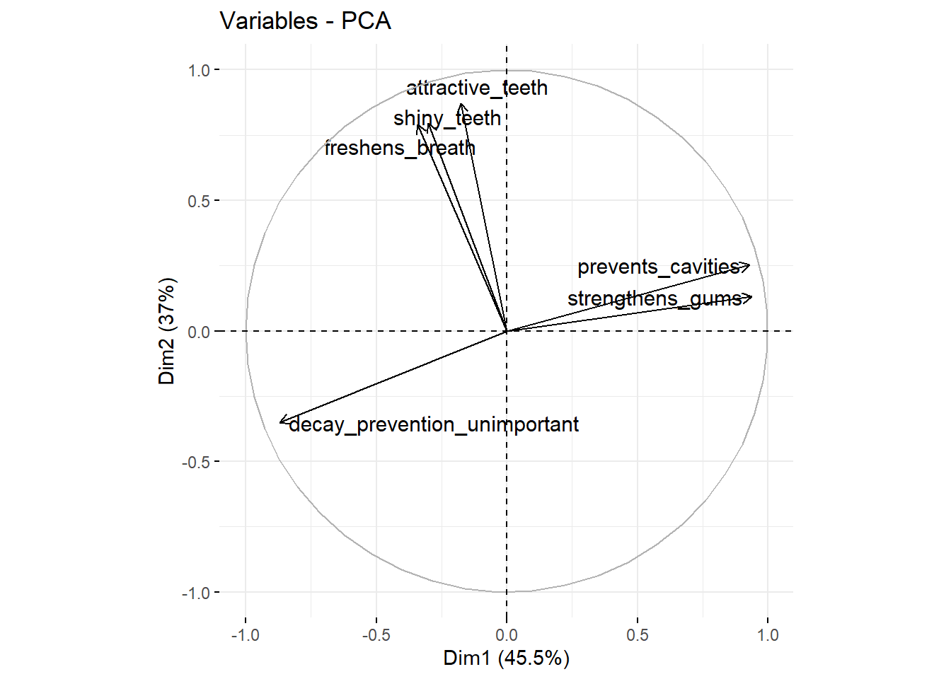
We see that attractive_teeth, shiny_teeth, freshens_breath have high scores on the second factor (the X-axis Dim2). prevents_cavities and strengthens_gums have high scores on the second factor (the Y-axis Dim2) and decay_prevention_unimportant has a low score on this factor (this variable measures how unimportant prevention of decay is). We can also add the observations (the different consumers) to this plot:
toothpaste %>% # take dataset
  select(-consumer,-age,-gender) %>% # retain only the dimensions
  as.data.frame() %>% # convert into a data.frame object, otherwise PCA won't accept it
  PCA(ncp = 2, graph = FALSE) %>% # do a principal components analysis and retain 2 factors
  fviz_pca_biplot(repel = TRUE) # take this analysis and turn it into a visualization
## Warning: ggrepel: 6 unlabeled data points (too many overlaps). Consider increasing max.overlaps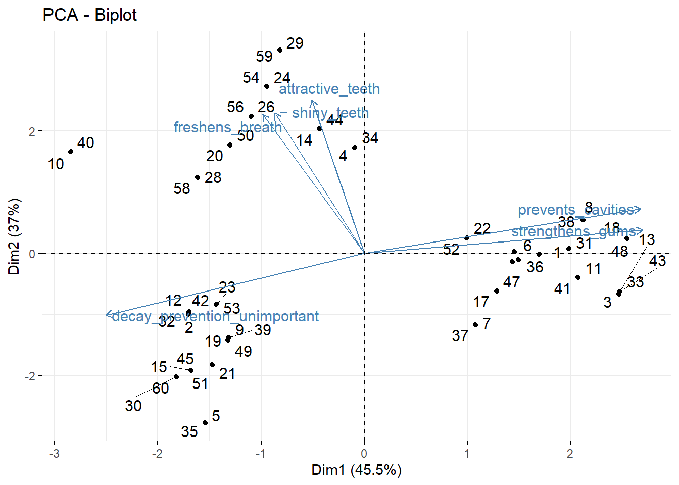
This is also called a biplot.