7 Cluster analysis for segmentation
In this chapter, you will learn how to carry out a cluster analysis and a linear discriminant analysis.
A cluster analysis works on a group of observations that differ from each other on a number of dimensions. It will find clusters of observations in the n-dimensional space such that the similarity of observations within clusters is as high as possible and the similarity of observations between clusters is as low as possible. You can always carry out a cluster analysis and you can ask for any number of clusters. The maximum number of clusters is the total number of observations. In that case each observation will be a cluster, but that would not be a very useful clustering, however. The goal of clustering is to find a small number of clusters that can be meaningfully described by their average scores on the n dimensions. In other words, the goal is to find different ‘profiles’ of observations.
Linear discriminant analysis tries to predict a categorical variable on the basis of a number of continuous or categorical independent variables. It is similar to logistic regression. We’ll use it to predict an observation’s cluster membership (as established by the cluster analysis) based on a few segmentation variables (i.e., other information we have on the observations that did not serve as input in the cluster analysis).
We will analyze data from 40 respondents who rated the importance of a number of store attributes when buying office equipment. We will use cluster analysis to find clusters of observations, in this case, clusters of respondents. These clusters will have different profiles (e.g., one cluster may attach importance to price and return policy, the other may attach importance to variety of choice and quality of service). We will then use linear discriminant analysis to test whether we can predict cluster membership (i.e., what type of office equipment shopper someone is) based on a number of respondent characteristics (e.g., their income).
7.1 Data
7.1.1 Import
We will analyze data from a survey in which 40 respondents were asked to rate the importance of a number of store attributes when buying equipment. Download the data here and import them into R:
library(tidyverse)
library(readxl)

equipment <- read_excel("segmentation_office.xlsx","SegmentationData") # Import the Excel file
7.1.2 Manipulate
equipment## # A tibble: 40 × 10
## respondent_id variety_of_choice electronics furniture quality_of_s…¹ low_p…² retur…³ profe…⁴ income age
## <dbl> <dbl> <dbl> <dbl> <dbl> <dbl> <dbl> <dbl> <dbl> <dbl>
## 1 1 8 6 6 3 2 2 1 40 45
## 2 2 6 3 1 4 7 8 0 20 41
## 3 3 6 1 2 4 9 6 0 20 31
## 4 4 8 3 3 4 8 7 1 30 37
## 5 5 4 6 3 9 2 5 1 45 56
## 6 6 8 4 3 5 10 6 1 35 28
## 7 7 7 2 2 2 8 7 1 45 30
## 8 8 7 5 7 2 2 3 0 15 58
## 9 9 7 7 5 1 5 4 0 45 55
## 10 10 8 4 0 4 9 8 0 45 23
## # … with 30 more rows, and abbreviated variable names ¹quality_of_service, ²low_prices, ³return_policy,
## # ⁴professional # Check out the dataWe have 10 columns or variables in our data:
respondent_idis an identifier for our observationsRespondents rated the importance of each of the following attributes on a 1-10 scale:
variety_of_choice,electronics,furniture,quality_of_service,low_prices,return_policy.professional: 1 for professionals, 0 for non-professionalsincome: expressed in thousands of dollarsage
The cluster analysis will try to identify clusters with similar patterns of ratings. Linear discriminant analysis will then predict cluster membership based on segmentation variables (professional, income, and age).
As always, let’s factorize the variables that should be treated as categorical:
equipment <- equipment %>%
  mutate(respondent_id = factor(respondent_id),
         professional = factor(professional, labels = c("non-professional","professional")))
7.1.3 Recap: importing & manipulating
Here’s what we’ve done so far, in one orderly sequence of piped operations (download the data here):
library(tidyverse)
library(readxl)

equipment <- read_excel("segmentation_office.xlsx","SegmentationData") %>%
  mutate(respondent_id = factor(respondent_id),
         professional = factor(professional, labels = c("non-professional","professional")))
7.2 Cluster analysis
We will first carry out a hierarchical cluster analysis to find the optimal number of clusters. After that, we will carry out a non-hierarchical cluster analysis and request the number of clusters deemed optimal by the hierarchical cluster analysis. The variables that will serve as input to the cluster analysis are the importance ratings of the store attributes.
7.2.1 Standardizing or not?
The first step in a cluster analysis is deciding whether to standardize the input variables. Standardizing is not necessary when the input variables are measured on the same scale or when the input variables are the coefficients obtained by a conjoint analysis. In other cases, standardizing is necessary.
In our example, all input variables are measured on the same scale and therefore standardizing is not necessary. If it were necessary, it can easily be done with mutate(newvar = scale(oldvar)).
7.3 Hierarchical clustering
Then, we create a new data set that only includes the input variables, i.e., the ratings:
cluster.data <- equipment %>%
  select(variety_of_choice, electronics, furniture, quality_of_service, low_prices, return_policy) # Select from the equipment dataset only the variables with the standardized ratings
We can now proceed with hierarchical clustering to determine the optimal number of clusters:
# The dist() function creates a dissimilarity matrix of our dataset and should be the first argument to the hclust() function.
# In the method argument, you can specify the method to use for clustering.
hierarchical.clustering <- hclust(dist(cluster.data), method = "ward.D")
The cluster analysis is stored in the hierarchical.clustering object and can easily be visualized by a dendogram:
plot(hierarchical.clustering)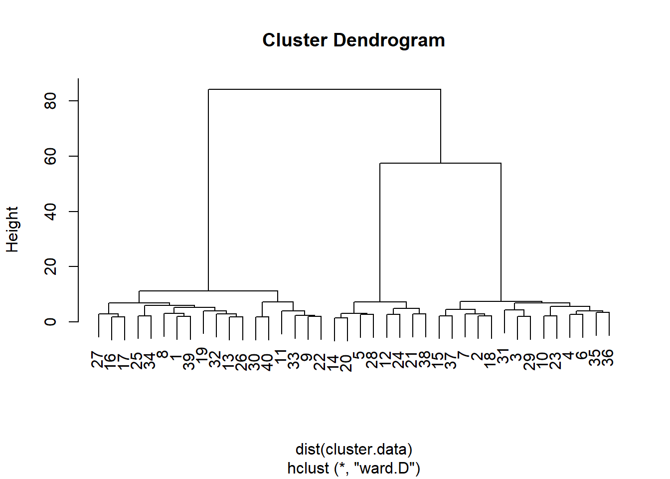
From this dendogram, it seems that that we can split the observations in either two, three, or six groups of observations. Let’s carry out a formal test, the Duda-Hart stopping rule, to see how many clusters we should retain. For this, we need to (install and) load the NbClust package:
install.packages("NbClust")
library(NbClust)
The Duda-Hart stopping rule table can be obtained as follows:
duda <- NbClust(cluster.data, distance = "euclidean", method = "ward.D2", max.nc = 9, index = "duda")
pseudot2 <- NbClust(cluster.data, distance = "euclidean", method = "ward.D2", max.nc = 9, index = "pseudot2")

duda$All.index
## 2 3 4 5 6 7 8 9
## 0.2997 0.7389 0.7540 0.5820 0.4229 0.7534 0.5899 0.7036pseudot2$All.index## 2 3 4 5 6 7 8 9
## 46.7352 5.6545 3.9145 4.3091 5.4591 3.2728 3.4757 2.9490The conventional wisdom for deciding the number of groups based on the Duda-Hart stopping rule is to find one of the largest Duda values that corresponds to a low pseudo-T2 value. However, you can also request the optimal number of clusters as suggested by the stopping rule:
duda$Best.nc## Number_clusters Value_Index
## 3.0000 0.7389In this case, the optimal number is three.
7.4 Non-hierarchical clustering
We now perform a non-hierarchical cluster analysis in which we ask for three clusters (as determined by the hierarchical cluster analysis):
# there is an element of randomness in cluster analysis
# this means that you will not always get the same output every time you do a cluster analysis
# if you do want to always get the same output, you need to fix R's random number generator with the set.seed command
set.seed(1)

# the nstart argument should be included and set to 25, but its explanation is out of the scope of this tutori al
kmeans.clustering <- kmeans(cluster.data, 3, nstart = 25)
Add to the equipment dataset a variable that indicates to which cluster an observation belongs:
equipment <- equipment %>%
  mutate(km.group = factor(kmeans.clustering$cluster, labels=c("cl1","cl2","cl3"))) # Factorize the cluster indicator from the kmeans.clustering data frame and add it to the equipment data frame.
Inspect the clusters:
equipment %>%
  group_by(km.group) %>% # group by cluster (km.group)
  summarise(count = n(),
            variety = mean(variety_of_choice),
            electronics = mean(electronics),
            furniture = mean(furniture),
            service = mean(quality_of_service),
            prices = mean(low_prices),
            return = mean(return_policy)) # Then ask for the number of respondents and for the means of the ratings.
## # A tibble: 3 × 8
## km.group count variety electronics furniture service prices return
## <fct> <int> <dbl> <dbl> <dbl> <dbl> <dbl> <dbl>
## 1 cl1 14 6.93 2.79 1.43 3.5 8.29 6.29
## 2 cl2 18 9.11 6.06 5.78 2.39 3.67 3.17
## 3 cl3 8 5 4.38 1.75 8.5 2.5 4.38We see that:
cluster 1 attaches more importance (than other clusters) to quality of service
cluster 2 attaches more importance to variety of choice
cluster 3 attaches more importance to low prices
We can also test whether there are significant differences between clusters in, for example, variety of choice. For this we use a one-way ANOVA:
# remotes::install_github("samuelfranssens/type3anova") # to install the type3anova package.
# You need the remotes package for this and the car package needs to be installed for the type3anova package to work
library(type3anova)
type3anova(lm(variety_of_choice ~ km.group, data=equipment))
## # A tibble: 3 × 6
## term ss df1 df2 f pvalue
## <chr> <dbl> <dbl> <int> <dbl> <dbl>
## 1 (Intercept) 1757. 1 37 1335. 0
## 2 km.group 101. 2 37 38.5 0
## 3 Residuals 48.7 37 37 NA NAThere are significant differences between clusters in importance attached to variety of choice, and this makes sense because the purpose of cluster analysis is to maximize between-cluster differences. Let’s follow this up with Tukey’s HSD to see exactly which means differ from each other:
TukeyHSD(aov(variety_of_choice ~ km.group, data=equipment),
         "km.group") # The first argument is an "aov" object, the second is our independent variable.
## Tukey multiple comparisons of means
## 95% family-wise confidence level
##
## Fit: aov(formula = variety_of_choice ~ km.group, data = equipment)
##
## $km.group
## diff lwr upr p adj
## cl2-cl1 2.182540 1.184332 3.1807470 0.0000145
## cl3-cl1 -1.928571 -3.170076 -0.6870668 0.0015154
## cl3-cl2 -4.111111 -5.301397 -2.9208248 0.0000000We see that in every pair of means, the difference is significant.
7.5 Canonical LDA
In real life, we usually don’t know what potential shoppers find important, but we do have an idea of, for example, their income, their age, and their professional status. It would therefore be useful to test how well we can predict cluster membership (profile of importance ratings) based on respondent characteristics (income, age, professional), which are also called segmentation variables. The predictive formula could then be used to predict the cluster membership of new potential shoppers. To find the right formula, we use linear discriminant analysis (LDA). But first let’s have a look at the averages of income, age, and professional per cluster:
equipment %>%
  group_by(km.group) %>% # Group equipment by cluster.
  summarize(income = mean(income),
            age = mean(age),
            professional = mean(as.numeric(professional)-1))
## # A tibble: 3 × 4
## km.group income age professional
## <fct> <dbl> <dbl> <dbl>
## 1 cl1 32.1 30.9 0.5
## 2 cl2 48.3 44.2 0.333
## 3 cl3 47.5 49 0.75# We cannot take the mean of professional because it is a factor variable.
# We therefore ask R to treat it as a numeric variable.
# Because the numeric version of professional takes on 1 and 2 as values, we deduct 1 so that the average indicates the percentage of people for which professional-1 is equal to 1, i.e., the percentage of professionals.We see that cluster 1 and 2 are somewhat similar in terms of income and age, but differ in the extent to which they consist of professionals. Cluster 3 differs from cluster 1 and 2 in that it is younger and less wealthy.
We can now use LDA to test how well we can predict cluster membership based on income, age, and professional:
library("MASS") # We need the MASS package. Install it first if needed.

lda.cluster3 <- lda(km.group ~ income + age + professional, data=equipment, CV=TRUE) # CV = TRUE ensures that we can store the prediction of the LDA in the following step
equipment <- equipment %>%
  mutate(class = factor(lda.cluster3$class, labels = c("lda1","lda2","lda3"))) # Save the prediction of the LDA as a factor. (The predictions are stored in lda.cluster3$class)
Let’s see how well the LDA has done:
ct <- table(equipment$km.group, equipment$class) # how many observations in each cluster were correctly predicted to be in that cluster by LDA?
ct
##
## lda1 lda2 lda3
## cl1 12 2 0
## cl2 3 12 3
## cl3 2 3 3We see, for example, that for the 14 observations in cluster 1, LDA correctly predicts that 12 are in cluster 1, but wrongly predicts that 2 are in cluster 2 and 0 are in cluster 3.
The overall prediction accuracy can be obtained as follows:
prop.table(ct) # get percentages##
## lda1 lda2 lda3
## cl1 0.300 0.050 0.000
## cl2 0.075 0.300 0.075
## cl3 0.050 0.075 0.075# add the percentages on the diagonal
sum(diag(prop.table(ct))) # Proportion correctly predicted## [1] 0.675Say we want to predict the cluster membership of new people for whom we only have income, age, and professional status, but not their cluster membership. We could look at the formula that the LDA has derived from the data of people for whom we did have cluster membership:
lda.cluster3.formula <- lda(km.group ~ income + age + professional, data=equipment, CV=FALSE) # CV = FALSE ensures that we view the formula that we can use for prediction
lda.cluster3.formula
## Call:
## lda(km.group ~ income + age + professional, data = equipment,
## CV = FALSE)
##
## Prior probabilities of groups:
## cl1 cl2 cl3
## 0.35 0.45 0.20
##
## Group means:
## income age professionalprofessional
## cl1 32.14286 30.92857 0.5000000
## cl2 48.33333 44.22222 0.3333333
## cl3 47.50000 49.00000 0.7500000
##
## Coefficients of linear discriminants:
## LD1 LD2
## income 0.02718175 -0.04456448
## age 0.08017200 0.03838914
## professionalprofessional 0.42492950 2.10385035
##
## Proportion of trace:
## LD1 LD2
## 0.7776 0.2224We see that the LDA has retained two discriminant dimensions (and this is where it differs from logistic regression, which is unidimensional). The first dimension explains 77.76 percent of the variance in km.group, the second dimension explains 22.24 percent of the variance in km.group. The table with coefficients gives us the formula for each dimension: Discriminant Score 1 = 0.03 \(\times\) income + 0.08 \(\times\) age + 0.42 \(\times\) professional & Discriminant Score 2 = -0.04 \(\times\) income + 0.04 \(\times\) age + 2.1 \(\times\) professional. To assign new observations to a certain cluster, we first need to calculate the average discriminant scores of the clusters and of each new observation (by filling in the (average) values of income, age, and professional of each cluster or observation in the discriminant functions), then calculate the geometrical distances between the discriminant scores of the new observations and the average discriminant scores of the clusters, and finally assign each observation to the cluster that is closest in geometrical space. This is quite a hassle, so we are lucky that R provides a simple way to do this.
Let’s create some new observations first:
# the tibble function can be used to create a new data frame
new_data <- tibble(income = c(65, 65, 35, 35), # to define a variable within the data frame, first provide the name of the variable (income), then provide the values
                   age = c(20, 35, 45, 60),
                   professional = c("professional","non-professional","non-professional","professional"))

# check out the new data:
new_data
## # A tibble: 4 × 3
## income age professional
## <dbl> <dbl> <chr>
## 1 65 20 professional
## 2 65 35 non-professional
## 3 35 45 non-professional
## 4 35 60 professionalNow let’s predict cluster membership for these “new” people:
new_data <- new_data %>%
  mutate(prediction = predict(lda.cluster3.formula, new_data)$class)
# Create a new column called prediction in the new_data data frame and store in that the prediction,
# accessed by $class, for the new_data based on the formula from the LDA based on the old data (use the LDA where CV = FALSE).

# have a look at the prediction:
new_data
## # A tibble: 4 × 4
## income age professional prediction
## <dbl> <dbl> <chr> <fct>
## 1 65 20 professional cl1
## 2 65 35 non-professional cl2
## 3 35 45 non-professional cl2
## 4 35 60 professional cl3