Chapter 3 Load the data
3.1 Uber data
For Uber, the operation is straightforward, thanks to the fread function from the data.table package. For this exercise, we will use the data.tablepackage to manipulate the data, due to its speed and conciseness compared to the alternative dplyr package.
Once loaded. we can have a glimpse at the Uber table :
## Classes 'data.table' and 'data.frame':   2409465 obs. of  13 variables:
##  $ year             : int  2019 2019 2019 2019 2019 2019 2019 2019 2019 2019 ...
##  $ month            : int  6 6 6 6 6 6 6 6 6 6 ...
##  $ day              : int  20 22 2 15 6 30 5 2 10 12 ...
##  $ hour             : int  18 0 13 0 19 4 19 13 0 9 ...
##  $ utc_timestamp    : chr  "2019-06-20T16:00:00.000Z" "2019-06-21T22:00:00.000Z" "2019-06-02T11:00:00.000Z" "2019-06-14T22:00:00.000Z" ...
##  $ segment_id       : chr  "f50b8a5ca0afcdd31eb48403172284dbc42f2aeb" "f50b8a5ca0afcdd31eb48403172284dbc42f2aeb" "f50b8a5ca0afcdd31eb48403172284dbc42f2aeb" "f50b8a5ca0afcdd31eb48403172284dbc42f2aeb" ...
##  $ start_junction_id: chr  "dc072f474bcbf30d75bd3b1e42974396af504bbb" "dc072f474bcbf30d75bd3b1e42974396af504bbb" "dc072f474bcbf30d75bd3b1e42974396af504bbb" "dc072f474bcbf30d75bd3b1e42974396af504bbb" ...
##  $ end_junction_id  : chr  "32c9d31816ecf0fde2586bab37995d06ad5f6f3e" "32c9d31816ecf0fde2586bab37995d06ad5f6f3e" "32c9d31816ecf0fde2586bab37995d06ad5f6f3e" "32c9d31816ecf0fde2586bab37995d06ad5f6f3e" ...
##  $ osm_way_id       : int  30709742 30709742 30709742 30709742 30709742 169753571 169753571 169753571 169753571 169753571 ...
##  $ osm_start_node_id:integer64 235637275 235637275 235637275 235637275 235637275 1813307792 1813307792 1813307792 ...
##  $ osm_end_node_id  :integer64 235637281 235637281 235637281 235637281 235637281 235637281 235637281 235637281 ...
##  $ speed_kph_mean   : num  48.1 37.3 30.5 39.9 42.9 ...
##  $ speed_kph_stddev : num  4.87 8.36 19.27 6.83 4.56 ...
##  - attr(*, ".internal.selfref")=<externalptr>
Nice gesture from Uber, the utc_timestamp has been also converted to other time dimensions (year,month,day,hour)
As stated on the Uber Movement metadata description, the columns segment_id, start_junction_id,end_junction_id correspond to the deprecated OSM (OpenStreetMap) identifiers for the ways (e.g. street/highways…) and nodes (junctions). Those 3 fields have been replace by the osm_way_id, osm_start_node_id, and osm_end_node_id.
In order to keep the process efficient, we can use our first data.table mutation operation on the table and remove those deprecated columns :
The operation does in fact take place by reference, i.e we do not copy the data.table, but modify it in place, which rquires less memory. We check that the removal operation took place :
## Classes 'data.table' and 'data.frame':   2409465 obs. of  10 variables:
##  $ year             : int  2019 2019 2019 2019 2019 2019 2019 2019 2019 2019 ...
##  $ month            : int  6 6 6 6 6 6 6 6 6 6 ...
##  $ day              : int  20 22 2 15 6 30 5 2 10 12 ...
##  $ hour             : int  18 0 13 0 19 4 19 13 0 9 ...
##  $ utc_timestamp    : chr  "2019-06-20T16:00:00.000Z" "2019-06-21T22:00:00.000Z" "2019-06-02T11:00:00.000Z" "2019-06-14T22:00:00.000Z" ...
##  $ osm_way_id       : int  30709742 30709742 30709742 30709742 30709742 169753571 169753571 169753571 169753571 169753571 ...
##  $ osm_start_node_id:integer64 235637275 235637275 235637275 235637275 235637275 1813307792 1813307792 1813307792 ...
##  $ osm_end_node_id  :integer64 235637281 235637281 235637281 235637281 235637281 235637281 235637281 235637281 ...
##  $ speed_kph_mean   : num  48.1 37.3 30.5 39.9 42.9 ...
##  $ speed_kph_stddev : num  4.87 8.36 19.27 6.83 4.56 ...
##  - attr(*, ".internal.selfref")=<externalptr>
Ok, the three deprecated columns have disappeared.
Now we can have a look at the structure of this table. If we understand correctly the description from Uber, each rows correspond to the aggregation of n trips per hour slot perosm_way_id (e.g. a part of the street), and per origin and destination (osm_start_node_id & osm_end_node_id).
Let’s take a sample of the table :
##                utc_timestamp osm_way_id osm_start_node_id osm_end_node_id
##  1: 2019-06-02T11:00:00.000Z  169753571        1813307792       235637281
##  2: 2019-06-02T11:00:00.000Z  169753571          26876458      2777147163
##  3: 2019-06-02T11:00:00.000Z  169753571        2238699687      2777147163
##  4: 2019-06-02T11:00:00.000Z  169753571         235637281      1813307792
##  5: 2019-06-02T11:00:00.000Z  169753571        2238699541      1813307792
##  6: 2019-06-02T11:00:00.000Z  169753571        2777147163        26876458
##  7: 2019-06-02T11:00:00.000Z  169753571        2777147163      2238699687
##  8: 2019-06-02T11:00:00.000Z  169753571        2777147147      2238699687
##  9: 2019-06-02T11:00:00.000Z  169753571        2238699687      2777147147
## 10: 2019-06-02T11:00:00.000Z  169753571        2238699582      2777147147
## 11: 2019-06-02T11:00:00.000Z  169753571        2777147147      2238699582
## 12: 2019-06-02T11:00:00.000Z  169753571        2238699541      2238699582
## 13: 2019-06-02T11:00:00.000Z  169753571        2238699582      2238699541
## 14: 2019-06-02T11:00:00.000Z  169753571        1813307792      2238699541
##     speed_kph_mean speed_kph_stddev
##  1:         21.007           17.470
##  2:         20.330           14.828
##  3:         16.792           13.527
##  4:         24.675           17.875
##  5:         26.493           20.579
##  6:         18.368           16.461
##  7:         24.360           18.828
##  8:         18.236            6.849
##  9:         26.236           20.184
## 10:         20.308           19.210
## 11:         26.810           21.513
## 12:         15.351           21.221
## 13:         26.450           21.985
## 14:         15.527           20.993
Let’s check if there are no duplicates :
##    mean_count std_count
## 1:          1         0
All right, the count value is always equal to 1.
From now on, as our aim is to evaluate the overall trips density and speed, as for the sake of simplicity, we keep our scope on the osm_way_id level rather the direction within the osm_way_id, which by the way, and we can figure it out on the Uber website, is not easy to visualize.
As we saw previously thanks to the “structure” str command, the Uber table as 2,409,465 rows.
Are those rows all valid, is there any missing data ? We can use the following operation to check that :
##                   col nok      ok   total
##  1:              year   0 2409465 2409465
##  2:             month   0 2409465 2409465
##  3:               day   0 2409465 2409465
##  4:              hour   0 2409465 2409465
##  5:     utc_timestamp   0 2409465 2409465
##  6:        osm_way_id   0 2409465 2409465
##  7: osm_start_node_id   0 2409465 2409465
##  8:   osm_end_node_id   0 2409465 2409465
##  9:    speed_kph_mean   0 2409465 2409465
## 10:  speed_kph_stddev   0 2409465 2409465
What have we done ? we first select the DT.Uber table, insert a comma because we do not want to filter the rows, then create four columns :
col: we use thenamesfunction to retrieve the list of column names of all the data.table columns (.SDfor SubsetData)nok: we compute the sum of non valid entries per column (.is.naon.SD), and use an intermediary variable assignment with the help of the<-operator (see 3.4.1 in the R Quick Tutorial)ok: logically, this is the difference between number of rows (.N) and thenoktotal: the total number of rows.
One good news : this table seems to be clean.
One more thing with this DT.Uber : the utc_timestamp is of class character, but we want it to be of type POSIXct, which is the standard datetime format in R. For this, we use the lubridate package with its ymd_hms method :
## POSIXct[1:2409465], format: "2019-06-20 16:00:00" "2019-06-21 22:00:00" ...Alleluja, the parsing (i.e. conversion) from class character to POSIXT was painless, which is worth mentioning.
But, is this dataset really for June 2019 ?
##           min_datetime        max_datetime
## 1: 2019-05-31 22:00:00 2019-06-30 21:00:00
Seems so indeed.
Now we can set indexing on this table, in order to, similarly to the SQL indexes, speed up the operations :
3.2 OSM data
Now we can load the OSM shapefile for the ways elements, with the help of the sf package (which is considerably faster than the rgdal package for read operations)
What have we done ? What is a shapefile ? we can look at its structure :
## Classes 'sf', 'tbl_df', 'tbl' and 'data.frame':  165629 obs. of  11 variables:
##  $ osm_id  : chr  "4045150" "4045194" "4045220" "4045223" ...
##  $ code    : int  5122 5122 5122 5122 5113 5114 5114 5122 5114 5122 ...
##  $ fclass  : chr  "residential" "residential" "residential" "residential" ...
##  $ name    : chr  "Waldstraße" "Ursula-Goetze-Straße" "Hönower Straße" "Gundelfinger Straße" ...
##  $ ref     : chr  NA NA NA NA ...
##  $ oneway  : chr  "B" "B" "B" "F" ...
##  $ maxspeed: int  50 30 30 30 50 50 30 30 50 0 ...
##  $ layer   : num  0 0 0 0 0 0 0 0 0 0 ...
##  $ bridge  : chr  "F" "F" "F" "F" ...
##  $ tunnel  : chr  "F" "F" "F" "F" ...
##  $ geometry:sfc_LINESTRING of length 165629; first list element:  'XY' num [1:13, 1:2] 13.6 13.6 13.6 13.6 13.6 ...
##  - attr(*, "sf_column")= chr "geometry"
##  - attr(*, "agr")= Factor w/ 3 levels "constant","aggregate",..: NA NA NA NA NA NA NA NA NA NA
##   ..- attr(*, "names")= chr  "osm_id" "code" "fclass" "name" ...
Nice, we have here a table with the OSM_id which we can connect to the Uber osm_way_id, they are brothers !
But what kind of object is OSM_sf ?
## [1] "sf" "tbl_df" "tbl" "data.frame"Well, a combination of sf, tbl_df, tbl and data.frame
The last column geometry contains as its name figures, the coordinates of each way id (that means how to draw the street with the help of multiple coordinates).
To calm down our excitment, we can plot a part of this shapefile with the use of the filter method (we do not want to plot the 165629 Polygons of all the ways !)
Here we filter out the ways that are of class motorway and residential and the streets with names containing “Marx” :
plot(st_geometry(OSM_sf%>% filter(fclass=='motorway')),col='navy',reset=F)
plot(st_geometry(OSM_sf%>% filter(fclass=='residential')),col='lightblue',add=T)
plot(st_geometry(OSM_sf%>% filter(grepl('Marx',name))),col='red',add=T)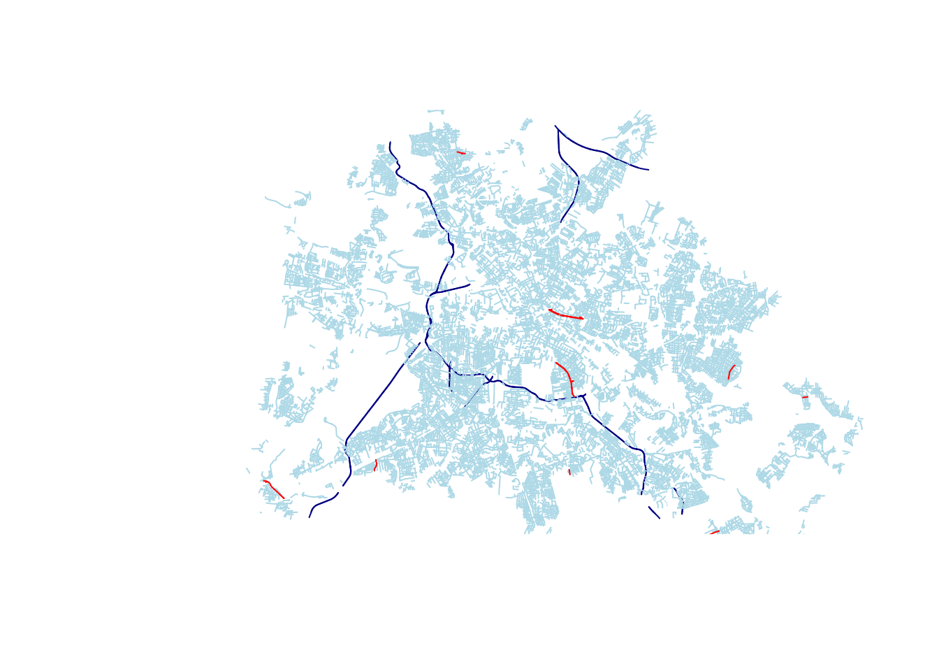
What we did here is first plot the motorway class, with the reset parameter set to FALSE, to allow the second and third plot calls with the residential class & name containing ‘Marx’ to be drawn on the same figure.
As a side note, we use the standard plot method of the sf package. One nice thing with sf is that you can also use the ggplot2 package for visualization. But in our case, the amount of elements to plot (>100000) make it very slow with ggplot2.
Now we that we have loaded our data in memory, we can start aggregating and merging those two datasets.