7 多元迴歸
以R語言內建的mtcars做多元迴歸。
7.1 資料的準備與檢視
7.1.1 讀入檔案
讀入mtcars檔案。mtcars是R內建的dataset,為1974年美國的Motor Trend雜誌對32種車款在11項設計與表現所做的整理,包含油耗量(mpg)、氣缸數(cyl)、排氣量(disp)、馬力(hp)、車體重量(wt)、加速時間(qsec)等。
##                    mpg cyl  disp  hp drat    wt  qsec vs am gear carb
## Mazda RX4         21.0   6 160.0 110 3.90 2.620 16.46  0  1    4    4
## Mazda RX4 Wag     21.0   6 160.0 110 3.90 2.875 17.02  0  1    4    4
## Datsun 710        22.8   4 108.0  93 3.85 2.320 18.61  1  1    4    1
## Hornet 4 Drive    21.4   6 258.0 110 3.08 3.215 19.44  1  0    3    1
## Hornet Sportabout 18.7   8 360.0 175 3.15 3.440 17.02  0  0    3    2
## Valiant           18.1   6 225.0 105 2.76 3.460 20.22  1  0    3    1
## Duster 360        14.3   8 360.0 245 3.21 3.570 15.84  0  0    3    4
## Merc 240D         24.4   4 146.7  62 3.69 3.190 20.00  1  0    4    2
## Merc 230          22.8   4 140.8  95 3.92 3.150 22.90  1  0    4    2
## Merc 280          19.2   6 167.6 123 3.92 3.440 18.30  1  0    4    4
7.1.2 檢視相關
先用plot()看各變項的關鍵性。
plot(mtcars[1:7])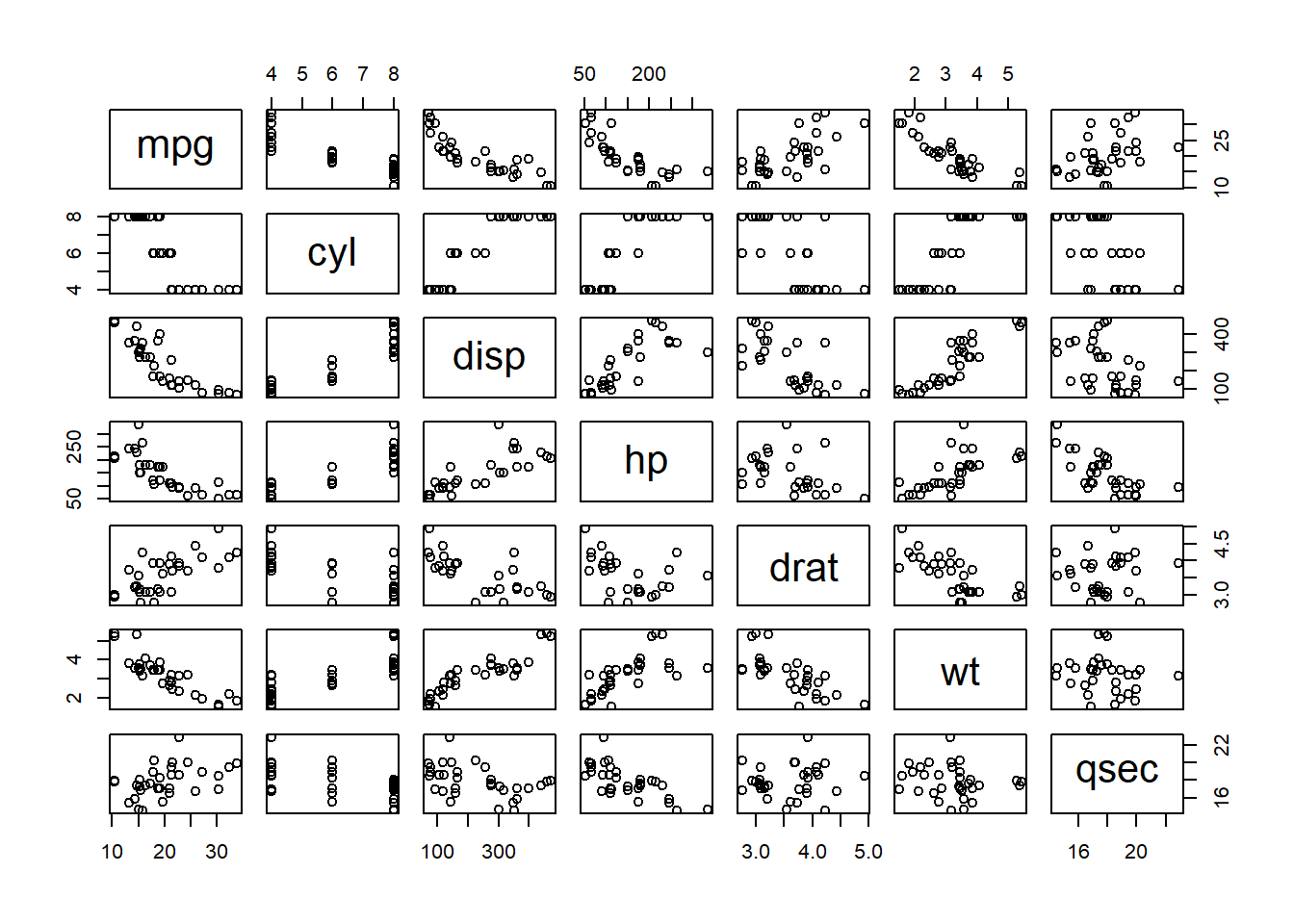
計算各變項的相關。
library(Hmisc)
rcorr(data.matrix(mtcars[1:7]))
## mpg cyl disp hp drat wt qsec
## mpg 1.00 -0.85 -0.85 -0.78 0.68 -0.87 0.42
## cyl -0.85 1.00 0.90 0.83 -0.70 0.78 -0.59
## disp -0.85 0.90 1.00 0.79 -0.71 0.89 -0.43
## hp -0.78 0.83 0.79 1.00 -0.45 0.66 -0.71
## drat 0.68 -0.70 -0.71 -0.45 1.00 -0.71 0.09
## wt -0.87 0.78 0.89 0.66 -0.71 1.00 -0.17
## qsec 0.42 -0.59 -0.43 -0.71 0.09 -0.17 1.00
##
## n= 32
##
##
## P
## mpg cyl disp hp drat wt qsec
## mpg 0.0000 0.0000 0.0000 0.0000 0.0000 0.0171
## cyl 0.0000 0.0000 0.0000 0.0000 0.0000 0.0004
## disp 0.0000 0.0000 0.0000 0.0000 0.0000 0.0131
## hp 0.0000 0.0000 0.0000 0.0100 0.0000 0.0000
## drat 0.0000 0.0000 0.0000 0.0100 0.0000 0.6196
## wt 0.0000 0.0000 0.0000 0.0000 0.0000 0.3389
## qsec 0.0171 0.0004 0.0131 0.0000 0.6196 0.33897.2 迴歸分析
7.2.1 簡單迴歸
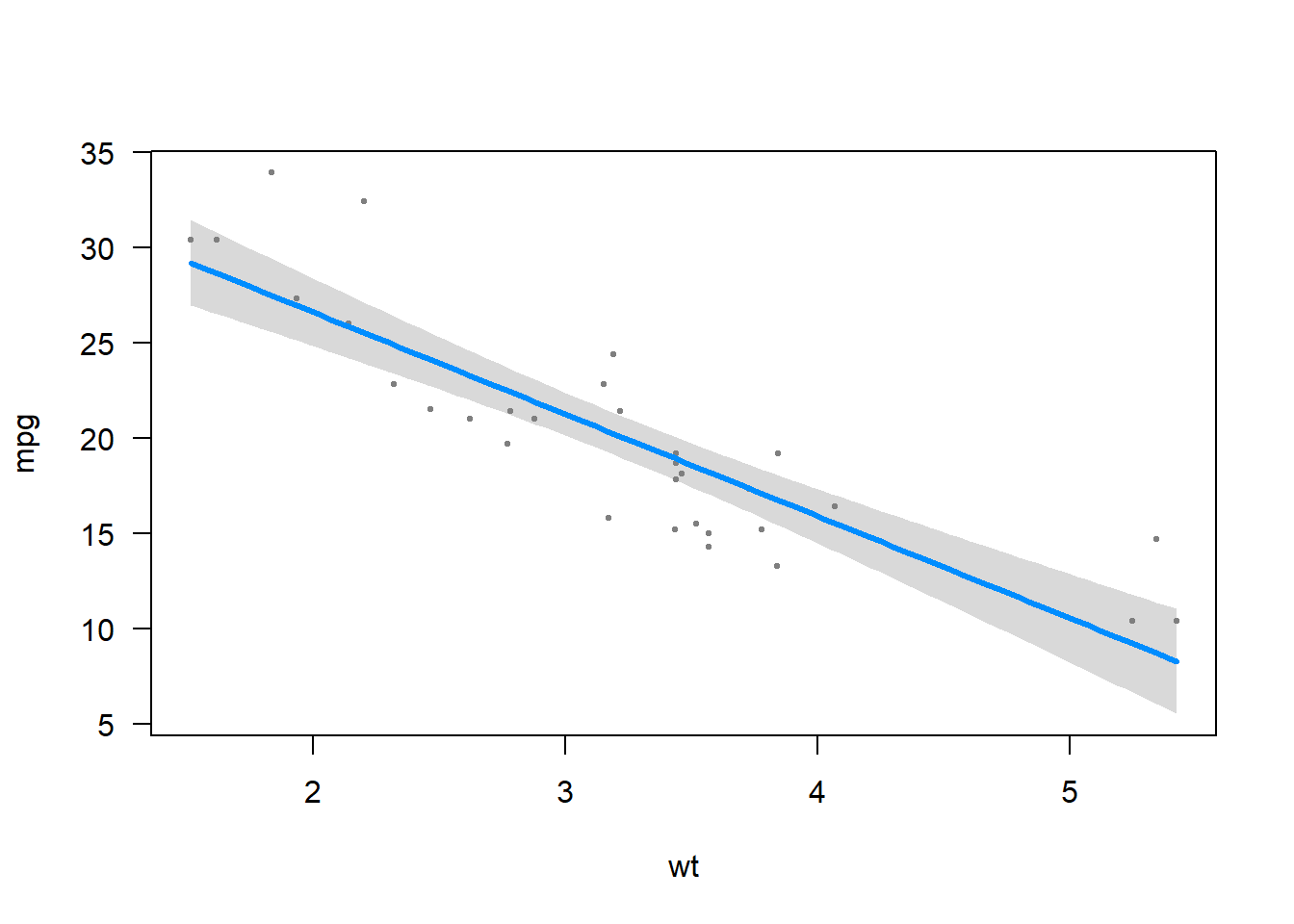
以lm()檢驗是否可以用車體重量(wt)預測油耗量(mpg)。結果顯示R-square = 0.75,F(1,30) = 91.38,p<.001,F檢定顯著,模型有良好解釋力。迴歸式為 mpg = -5.3445*wt + 37.2851。
##
## Call:
## lm(formula = mpg ~ wt, data = mtcars)
##
## Residuals:
##     Min      1Q  Median      3Q     Max
## -4.5432 -2.3647 -0.1252  1.4096  6.8727
##
## Coefficients:
##             Estimate Std. Error t value Pr(>|t|)
## (Intercept)  37.2851     1.8776  19.858  < 2e-16 ***
## wt           -5.3445     0.5591  -9.559 1.29e-10 ***
## ---
## Signif. codes:  0 '***' 0.001 '**' 0.01 '*' 0.05 '.' 0.1 ' ' 1
##
## Residual standard error: 3.046 on 30 degrees of freedom
## Multiple R-squared:  0.7528, Adjusted R-squared:  0.7446
## F-statistic: 91.38 on 1 and 30 DF,  p-value: 1.294e-10
以package visreg的visreg()函數來畫迴歸線。
7.2.2 多元迴歸
以車體重量(wt)、馬力(hp)和排氣量(disp)來預測油耗量(mpg)。相關分析顯示三個預測項與油耗量皆為負相關。
以lm()來做迴歸分析,迴歸分析結果顯示,R-square = 0.8268,F(3,28) = 44.57, p < .01。disp沒有顯著。
model.mpg.whd <- update(model.mpg.wt, .~. + hp + disp, data=mtcars)
model.mpg.whd <- lm(mpg ~ wt + hp + disp, data = mtcars)
summary(model.mpg.whd)
##
## Call:
## lm(formula = mpg ~ wt + hp + disp, data = mtcars)
##
## Residuals:
## Min 1Q Median 3Q Max
## -3.891 -1.640 -0.172 1.061 5.861
##
## Coefficients:
## Estimate Std. Error t value Pr(>|t|)
## (Intercept) 37.105505 2.110815 17.579 < 2e-16 ***
## wt -3.800891 1.066191 -3.565 0.00133 **
## hp -0.031157 0.011436 -2.724 0.01097 *
## disp -0.000937 0.010350 -0.091 0.92851
## ---
## Signif. codes: 0 '***' 0.001 '**' 0.01 '*' 0.05 '.' 0.1 ' ' 1
##
## Residual standard error: 2.639 on 28 degrees of freedom
## Multiple R-squared: 0.8268, Adjusted R-squared: 0.8083
## F-statistic: 44.57 on 3 and 28 DF, p-value: 8.65e-11若想進一步看淨相關和半淨相關,可用pcor()做淨相關(partial correlation)、用spcor()做半淨相關(semi-partial correlation)。淨相關結果顯示,三變項皆顯著相關,all ps < .05。
##         mpg     wt     hp   disp
## mpg   1.000 -0.559 -0.458 -0.017
## wt   -0.559  1.000 -0.370  0.651
## hp   -0.458 -0.370  1.000  0.521
## disp -0.017 0.651 0.521 1.000## mpg wt hp disp
## mpg 0.000 0.001 0.011 0.929
## wt 0.001 0.000 0.044 0.000
## hp 0.011 0.044 0.000 0.003
## disp 0.929 0.000 0.003 0.000半淨相關結果顯示,僅wt顯著相關。
##         mpg     wt     hp   disp
## mpg   1.000 -0.280 -0.214 -0.007
## wt   -0.254  1.000 -0.150  0.323
## hp   -0.277 -0.214  1.000  0.328
## disp -0.006 0.317 0.226 1.000## mpg wt hp disp
## mpg 0.000 0.133 0.256 0.970
## wt 0.176 0.000 0.429 0.081
## hp 0.139 0.256 0.000 0.076
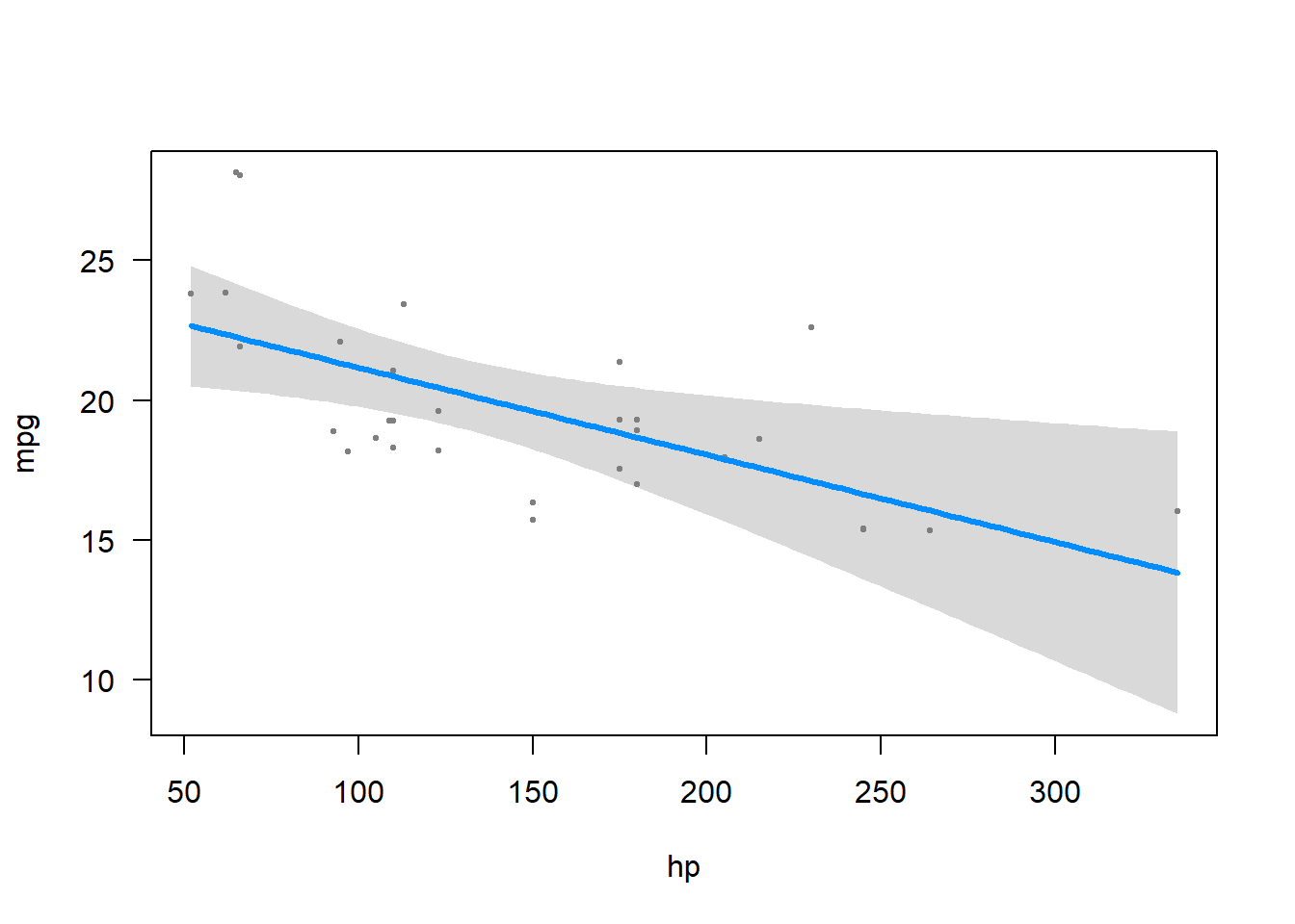
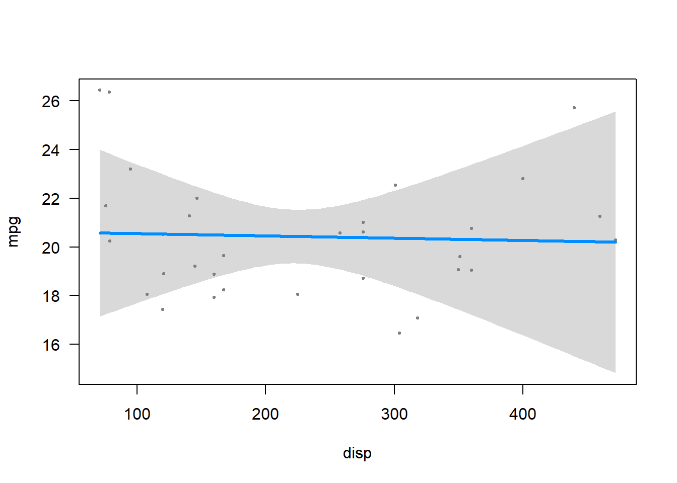
## disp 0.974 0.088 0.230 0.000看各變項對mpg的關係。
visreg(model.mpg.whd)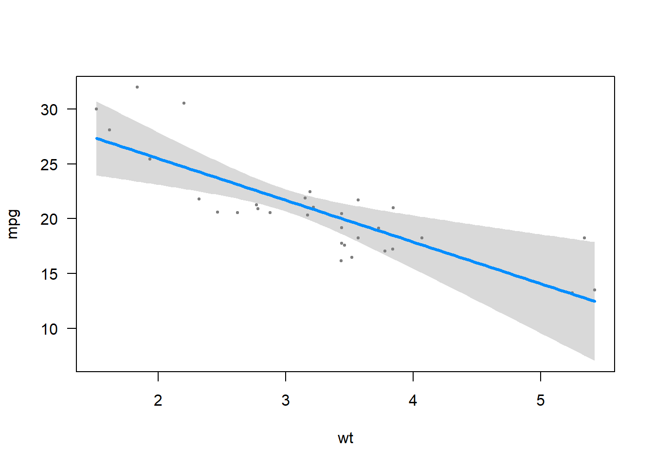
以predict()來做預測。
predict(model.mpg.whd,
        new = data.frame(wt = 5, hp = 250, disp = 300, am = "Manual"),
        interval = "confidence",
        level = .95
)
## fit lwr upr
## 1 10.03081 6.335154 13.726477.2.3 迴歸模型的比較
以ANOVA()來比較兩個迴歸模型。結果顯示三預測項的模型顯著優於一預測項模型。F(2, 83.33) = 5.98, p<.001。
anova(model.mpg.wt, model.mpg.whd)## Analysis of Variance Table
##
## Model 1: mpg ~ wt
## Model 2: mpg ~ wt + hp + disp
## Res.Df RSS Df Sum of Sq F Pr(>F)
## 1 30 278.32
## 2 28 194.99 2 83.331 5.983 0.006863 **
## ---
## Signif. codes: 0 '***' 0.001 '**' 0.01 '*' 0.05 '.' 0.1 ' ' 1用AIC()來看兩個模型的AIC(Akaike information criterion)。結果顯示相較於一個預測項時,以三個預測項來預測mpg時,AIC有下降。
AIC(model.mpg.wt)## [1] 166.0294
AIC(model.mpg.whd)## [1] 158.6437.3 迴歸假設的檢驗
檢驗資料是否符合迴歸分析的假設。
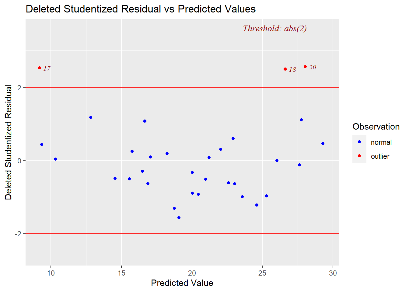
7.3.1 極端數值的影響
standardize resuduals和studentize residuals。
library(olsrr)
ols_plot_resid_stand(model.mpg.whd)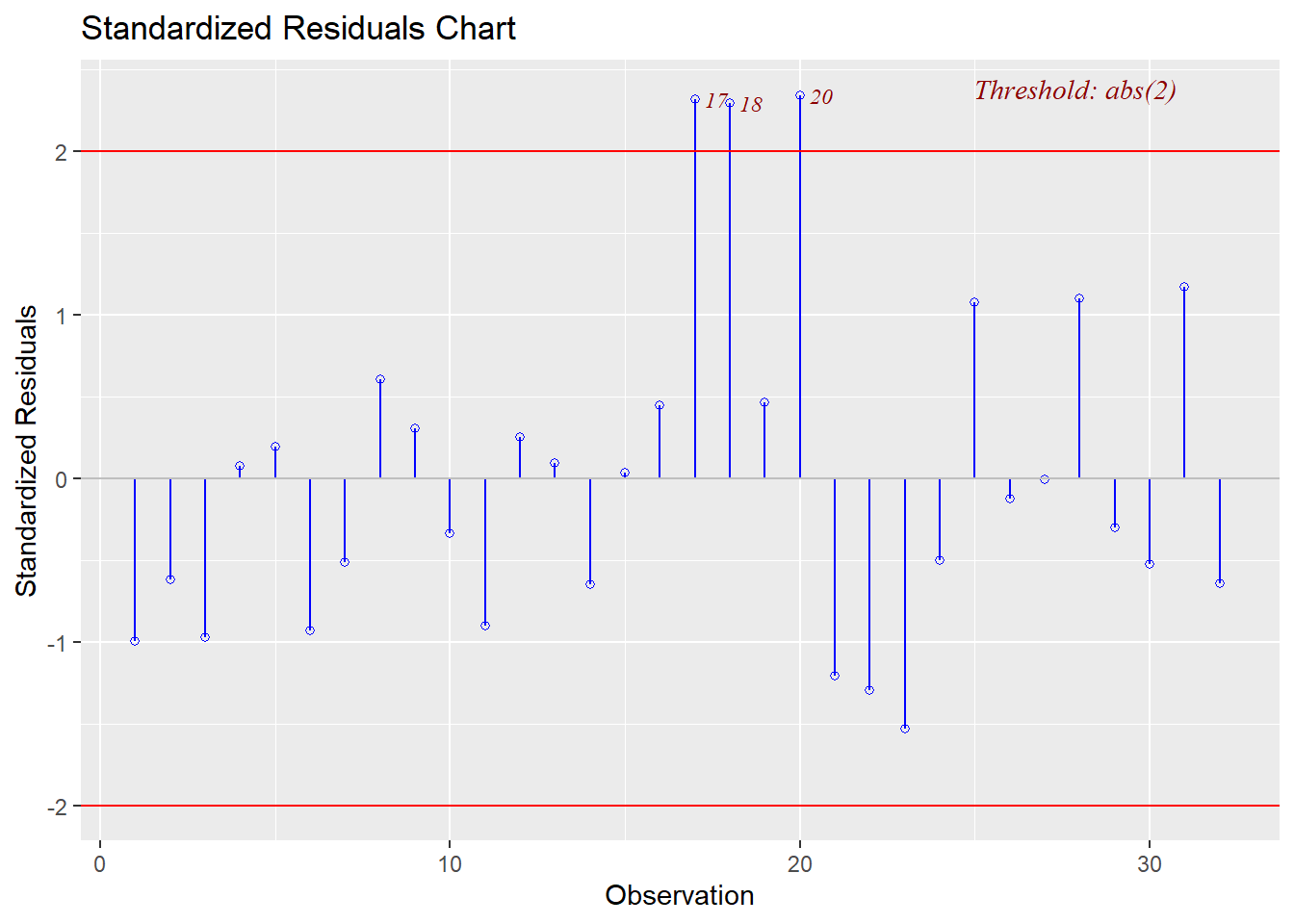
ols_plot_resid_stud(model.mpg.whd)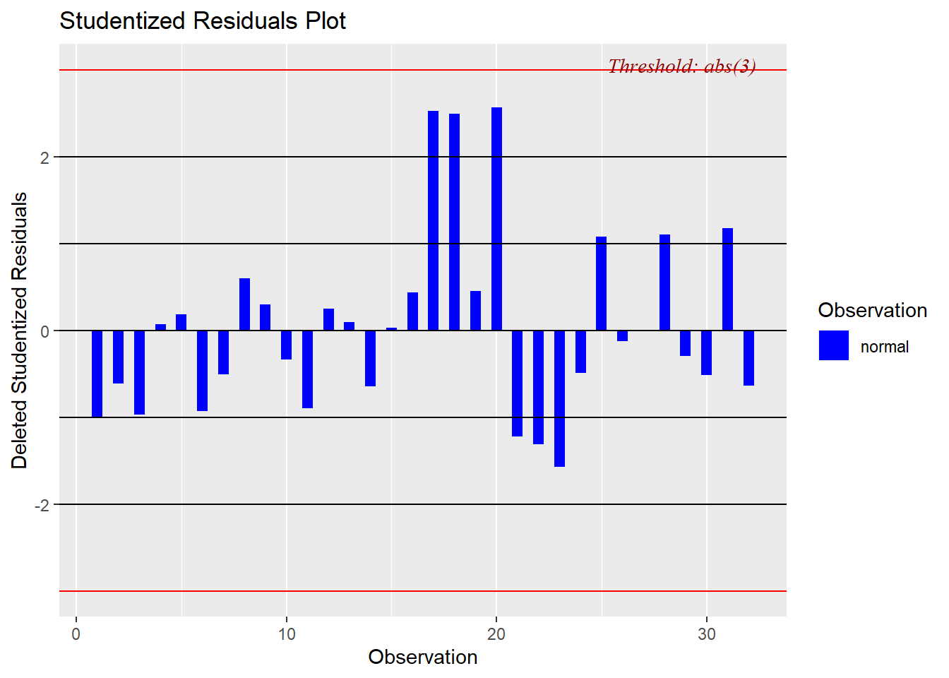
極端數值移除後對迴歸式的影響。
ols_plot_dfbetas(model.mpg.whd)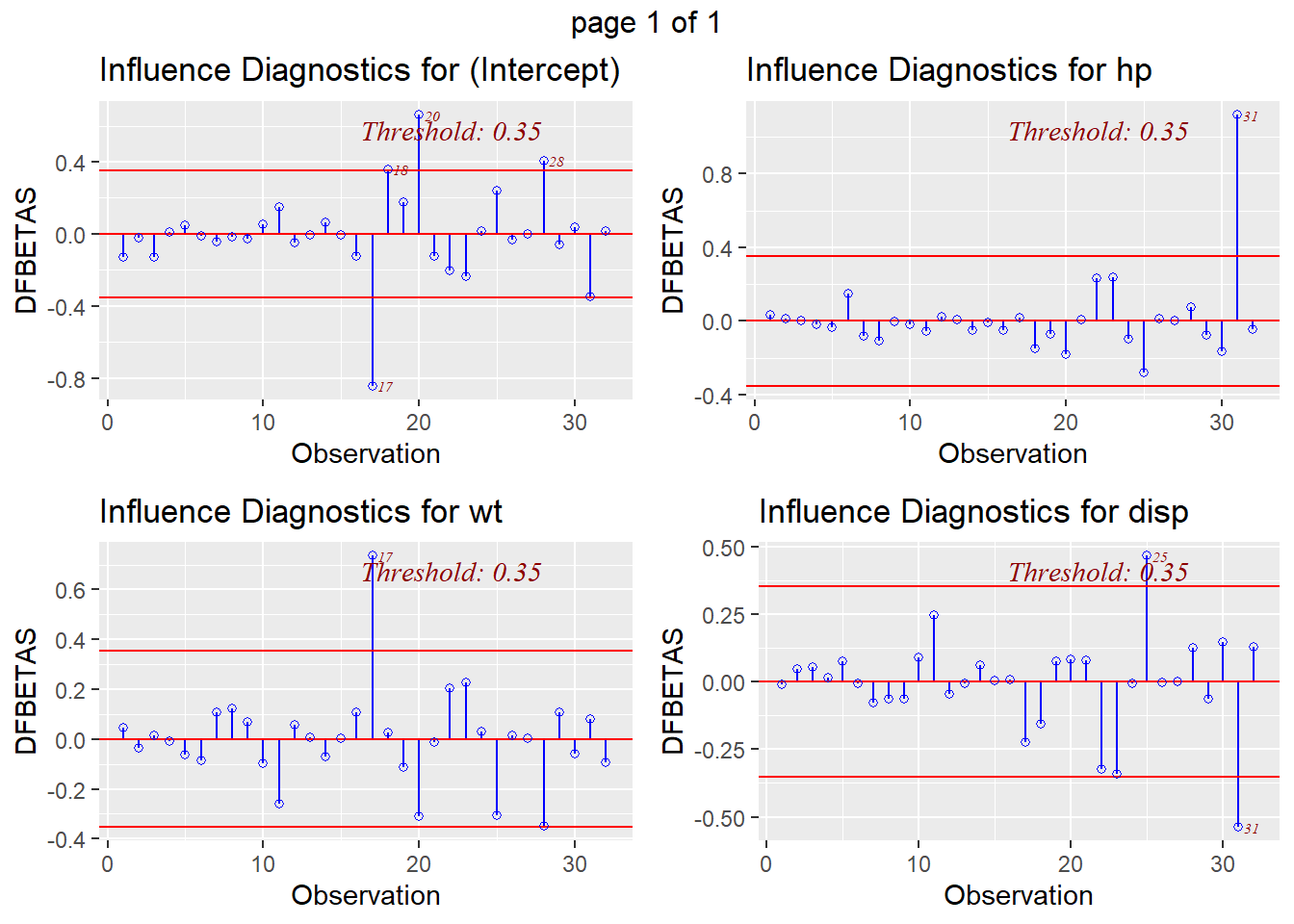
ols_plot_dffits(model.mpg.whd)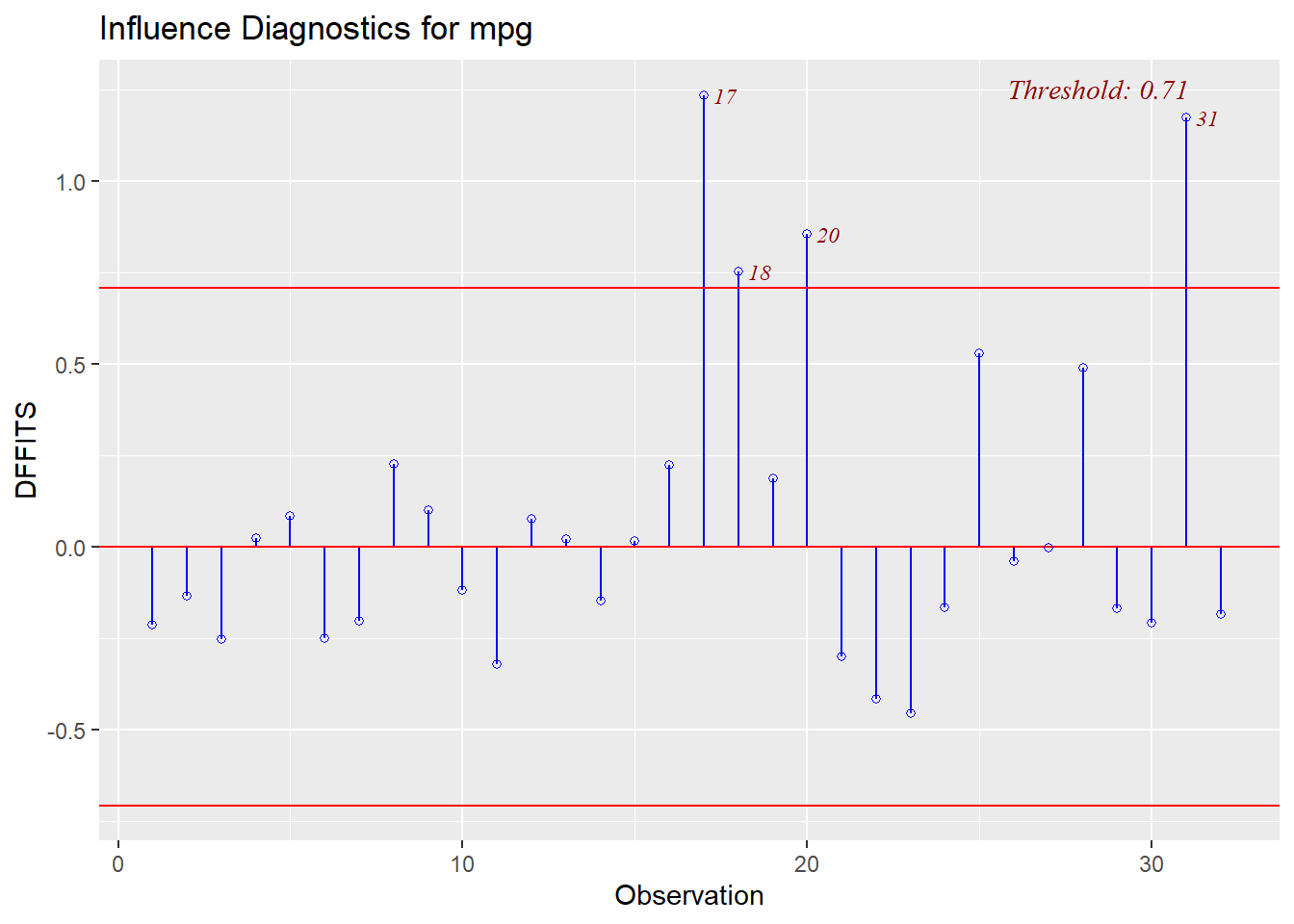
以Cook’s distance看極端數值對整個模型的影響。
ols_plot_cooksd_bar(model.mpg.whd)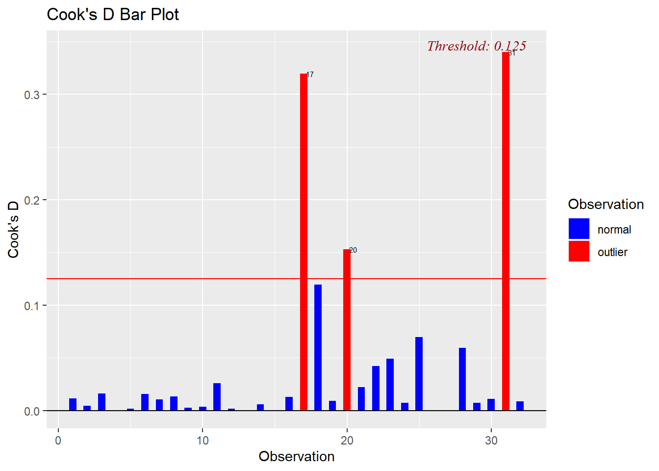
ols_plot_cooksd_chart(model.mpg.whd)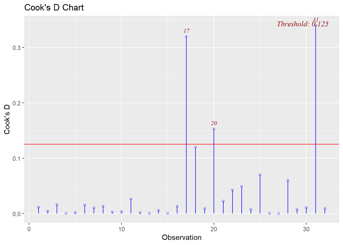
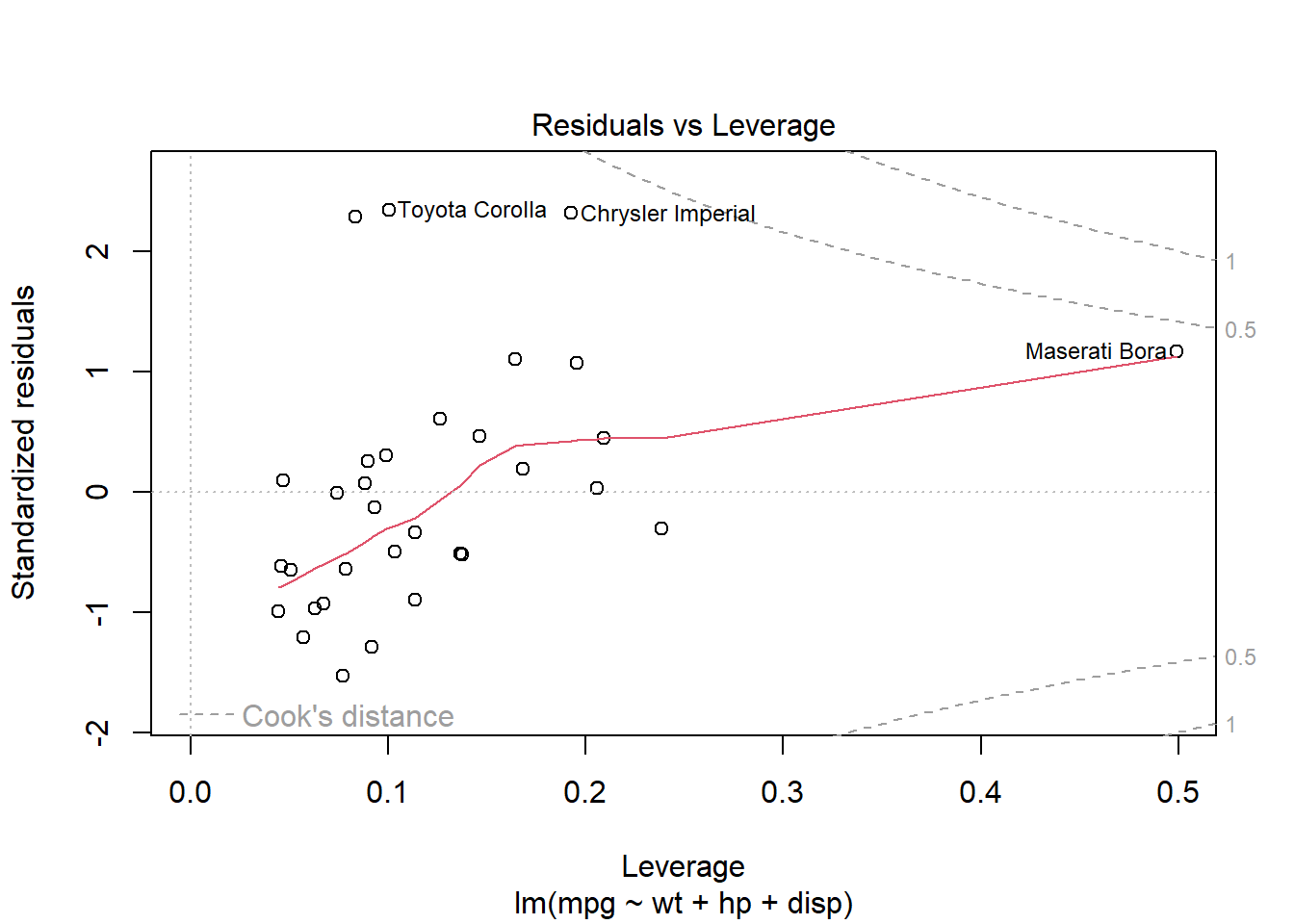
看residual和leverage。
library(olsrr)
ols_plot_resid_lev(model.mpg.whd)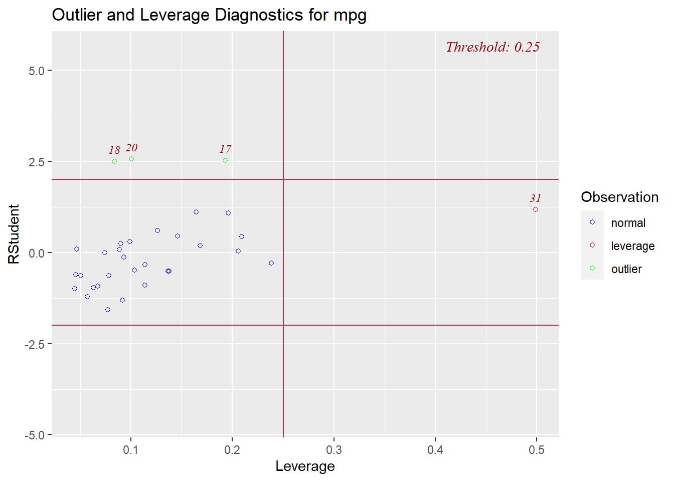
7.3.3 共線性multicollinearity的檢驗
看vif和tolerance。最大的VIF大於10要注意、平均的VIF大於1可能有偏誤;tolerance小於0.1要注意、tolerance小於0.2可能有問題。
##       wt       hp     disp
## 4.844618 2.736633 7.324517
1/vif(model.mpg.whd)## wt hp disp
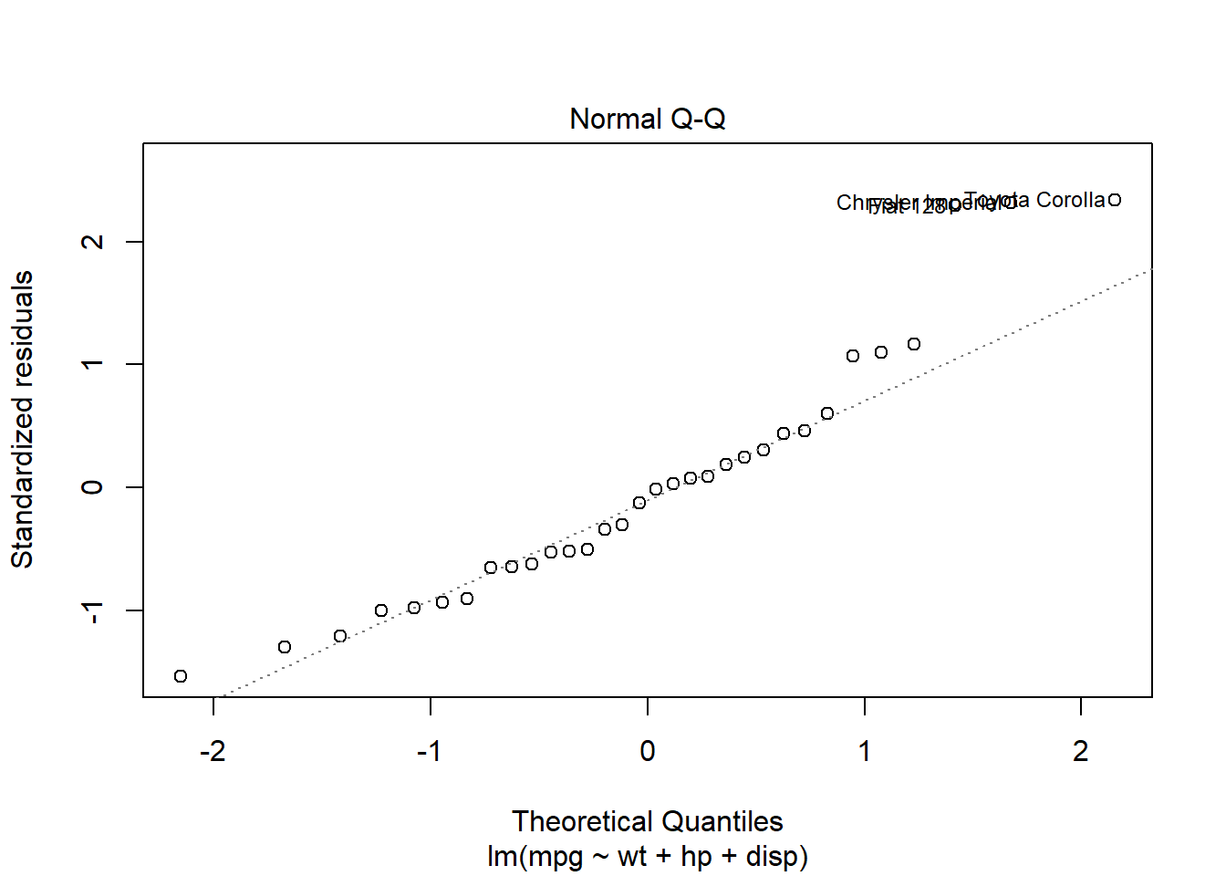
## 0.2064146 0.3654126 0.13652787.3.4 誤差常態的檢定
residuals常態分配的檢定。
shapiro.test(residuals(model.mpg.whd))##
## Shapiro-Wilk normality test
##
## data: residuals(model.mpg.whd)
## W = 0.92734, p-value = 0.033057.3.5 自相關檢驗
用Durbin-Watson test看是否有autocorrelation。
##  lag Autocorrelation D-W Statistic p-value
##    1       0.2926117      1.367284    0.03
##  Alternative hypothesis: rho != 0
durbinWatsonTest(model.mpg.whd)## lag Autocorrelation D-W Statistic p-value
## 1 0.2926117 1.367284 0.04
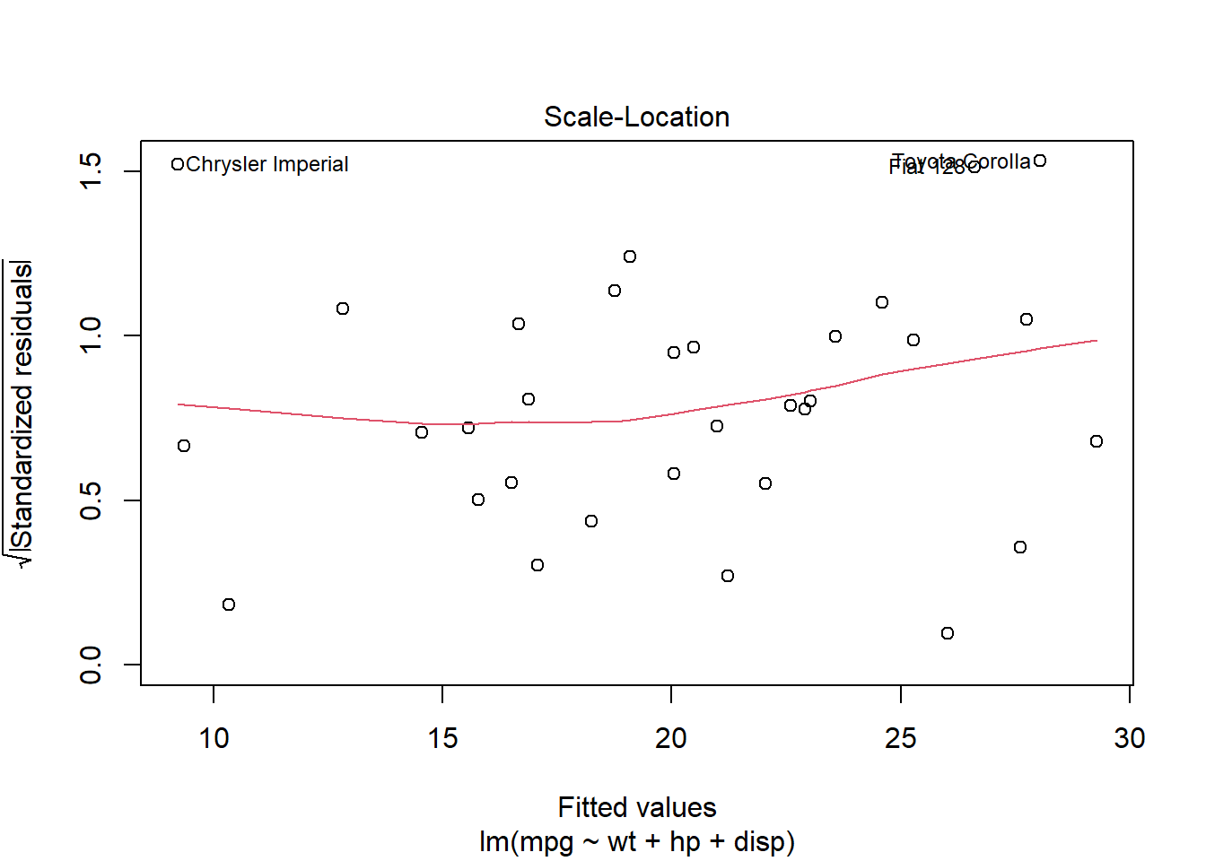
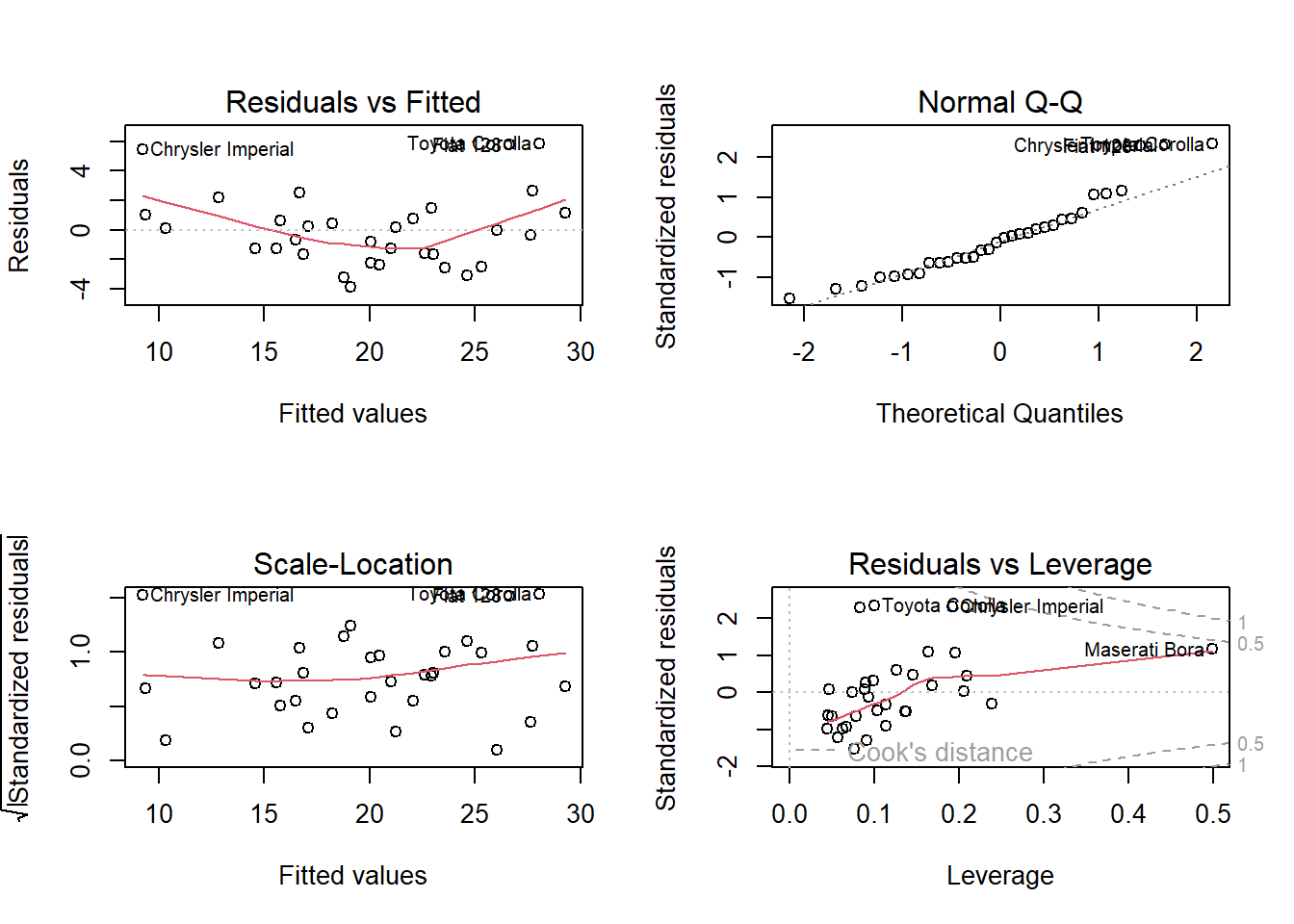
## Alternative hypothesis: rho != 07.3.6 綜合檢驗
可用內建的plot()功能一次看上述檢驗。若加which=1:6可看更多。
plot(model.mpg.whd)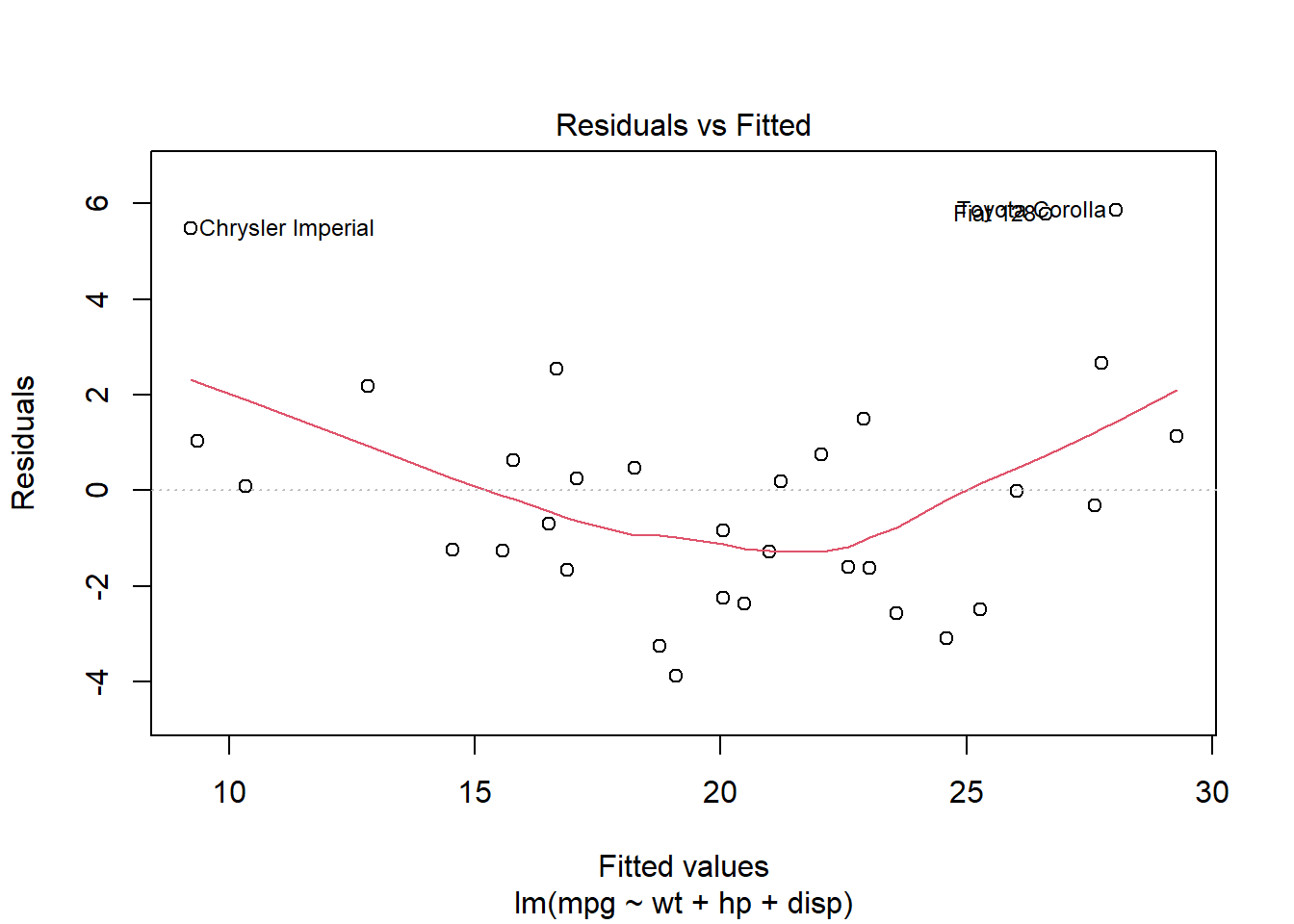
也可以將圖表放在一起看。
或以performance這個package來看迴歸的假設。
library(performance)
library(see)
library(patchwork)
check_model(model.mpg.whd)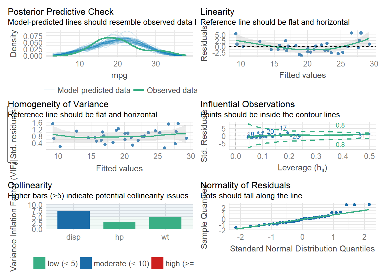
計算各統計量並儲存。
mtcars$residuals <- resid(model.mpg.whd)
mtcars$standardized.residuals <- rstandard(model.mpg.whd)
mtcars$studentized.residuals <- rstudent(model.mpg.whd)
mtcars$cooks.distance <- cooks.distance(model.mpg.whd)
mtcars$leverage <- hatvalues(model.mpg.whd)
mtcars <- cbind(mtcars, dfbetas(model.mpg.whd))
names(mtcars)[12:15] <- c('db_intercept', 'db_wt', 'db_hp', 'db_disp')
mtcars$dffit <- dffits(model.mpg.whd)
mtcars$fitted <- fitted(model.mpg.whd)
7.4 逐步迴歸
7.4.1 前向法
用lm()做逐步回歸。以下為前向法。
mtcars2 <- mtcars[c(1,6,4,3)]
nullM <- lm(mpg ~ 1, data = mtcars2)
fullM <- lm(mpg ~ ., data = mtcars2)
forM <- step(nullM, scope=list(lower=nullM, upper=fullM), direction="forward")
## Start: AIC=115.94
## mpg ~ 1
##
## Df Sum of Sq RSS AIC
## + wt 1 847.73 278.32 73.217
## + disp 1 808.89 317.16 77.397
## + hp 1 678.37 447.67 88.427
## <none> 1126.05 115.943
##
## Step: AIC=73.22
## mpg ~ wt
##
## Df Sum of Sq RSS AIC
## + hp 1 83.274 195.05 63.840
## + disp 1 31.639 246.68 71.356
## <none> 278.32 73.217
##
## Step: AIC=63.84
## mpg ~ wt + hp
##
## Df Sum of Sq RSS AIC
## <none> 195.05 63.840
## + disp 1 0.05708 194.99 65.831
summary(forM)##
## Call:
## lm(formula = mpg ~ wt + hp, data = mtcars2)
##
## Residuals:
## Min 1Q Median 3Q Max
## -3.941 -1.600 -0.182 1.050 5.854
##
## Coefficients:
## Estimate Std. Error t value Pr(>|t|)
## (Intercept) 37.22727 1.59879 23.285 < 2e-16 ***
## wt -3.87783 0.63273 -6.129 1.12e-06 ***
## hp -0.03177 0.00903 -3.519 0.00145 **
## ---
## Signif. codes: 0 '***' 0.001 '**' 0.01 '*' 0.05 '.' 0.1 ' ' 1
##
## Residual standard error: 2.593 on 29 degrees of freedom
## Multiple R-squared: 0.8268, Adjusted R-squared: 0.8148
## F-statistic: 69.21 on 2 and 29 DF, p-value: 9.109e-127.4.2 後向法
backward method。
fullM <- lm(mpg ~ ., data = mtcars2)
# backM <- step(fullM, scope=list(upper=fullM), direction='backward') # 完整寫法
backM <- step(fullM, direction='backward')
## Start: AIC=65.83
## mpg ~ wt + hp + disp
##
## Df Sum of Sq RSS AIC
## - disp 1 0.057 195.05 63.840
## <none> 194.99 65.831
## - hp 1 51.692 246.68 71.356
## - wt 1 88.503 283.49 75.806
##
## Step: AIC=63.84
## mpg ~ wt + hp
##
## Df Sum of Sq RSS AIC
## <none> 195.05 63.840
## - hp 1 83.274 278.32 73.217
## - wt 1 252.627 447.67 88.427
summary(backM)##
## Call:
## lm(formula = mpg ~ wt + hp, data = mtcars2)
##
## Residuals:
## Min 1Q Median 3Q Max
## -3.941 -1.600 -0.182 1.050 5.854
##
## Coefficients:
## Estimate Std. Error t value Pr(>|t|)
## (Intercept) 37.22727 1.59879 23.285 < 2e-16 ***
## wt -3.87783 0.63273 -6.129 1.12e-06 ***
## hp -0.03177 0.00903 -3.519 0.00145 **
## ---
## Signif. codes: 0 '***' 0.001 '**' 0.01 '*' 0.05 '.' 0.1 ' ' 1
##
## Residual standard error: 2.593 on 29 degrees of freedom
## Multiple R-squared: 0.8268, Adjusted R-squared: 0.8148
## F-statistic: 69.21 on 2 and 29 DF, p-value: 9.109e-127.4.3 逐步法
Stepwise method。
7.4.3.1 從full model開始
fullM <- lm(mpg ~ ., data = mtcars2)
# stepM1 <- step(fullM, scope = list(upper=fullM), direction="both") # 完整寫法
stepM1 <- step(fullM, direction="both") ## Start: AIC=65.83
## mpg ~ wt + hp + disp
##
## Df Sum of Sq RSS AIC
## - disp 1 0.057 195.05 63.840
## <none> 194.99 65.831
## - hp 1 51.692 246.68 71.356
## - wt 1 88.503 283.49 75.806
##
## Step: AIC=63.84
## mpg ~ wt + hp
##
## Df Sum of Sq RSS AIC
## <none> 195.05 63.840
## + disp 1 0.057 194.99 65.831
## - hp 1 83.274 278.32 73.217
## - wt 1 252.627 447.67 88.4277.4.3.2 從null model開始
結果可能會與從full model開始不同。
nullM <- lm(mpg ~ 1, data = mtcars2)
stepM2 <- step(nullM, scope = list(upper=fullM), direction="both")## Start: AIC=115.94
## mpg ~ 1
##
## Df Sum of Sq RSS AIC
## + wt 1 847.73 278.32 73.217
## + disp 1 808.89 317.16 77.397
## + hp 1 678.37 447.67 88.427
## <none> 1126.05 115.943
##
## Step: AIC=73.22
## mpg ~ wt
##
## Df Sum of Sq RSS AIC
## + hp 1 83.27 195.05 63.840
## + disp 1 31.64 246.68 71.356
## <none> 278.32 73.217
## - wt 1 847.73 1126.05 115.943
##
## Step: AIC=63.84
## mpg ~ wt + hp
##
## Df Sum of Sq RSS AIC
## <none> 195.05 63.840
## + disp 1 0.057 194.99 65.831
## - hp 1 83.274 278.32 73.217
## - wt 1 252.627 447.67 88.427
summary(stepM1)##
## Call:
## lm(formula = mpg ~ wt + hp, data = mtcars2)
##
## Residuals:
## Min 1Q Median 3Q Max
## -3.941 -1.600 -0.182 1.050 5.854
##
## Coefficients:
## Estimate Std. Error t value Pr(>|t|)
## (Intercept) 37.22727 1.59879 23.285 < 2e-16 ***
## wt -3.87783 0.63273 -6.129 1.12e-06 ***
## hp -0.03177 0.00903 -3.519 0.00145 **
## ---
## Signif. codes: 0 '***' 0.001 '**' 0.01 '*' 0.05 '.' 0.1 ' ' 1
##
## Residual standard error: 2.593 on 29 degrees of freedom
## Multiple R-squared: 0.8268, Adjusted R-squared: 0.8148
## F-statistic: 69.21 on 2 and 29 DF, p-value: 9.109e-12
summary(stepM2)##
## Call:
## lm(formula = mpg ~ wt + hp, data = mtcars2)
##
## Residuals:
## Min 1Q Median 3Q Max
## -3.941 -1.600 -0.182 1.050 5.854
##
## Coefficients:
## Estimate Std. Error t value Pr(>|t|)
## (Intercept) 37.22727 1.59879 23.285 < 2e-16 ***
## wt -3.87783 0.63273 -6.129 1.12e-06 ***
## hp -0.03177 0.00903 -3.519 0.00145 **
## ---
## Signif. codes: 0 '***' 0.001 '**' 0.01 '*' 0.05 '.' 0.1 ' ' 1
##
## Residual standard error: 2.593 on 29 degrees of freedom
## Multiple R-squared: 0.8268, Adjusted R-squared: 0.8148
## F-statistic: 69.21 on 2 and 29 DF, p-value: 9.109e-127.4.3.3 另一種作法
可用stepAIC()來做逐步回歸。沒指定scope時會用backward;指定scope時會用both。可用direction來指定forward、backward或both。
## Start:  AIC=65.83
## mpg ~ wt + hp + disp
##
##        Df Sum of Sq    RSS    AIC
## - disp  1     0.057 195.05 63.840
## <none>              194.99 65.831
## - hp    1    51.692 246.68 71.356
## - wt    1    88.503 283.49 75.806
##
## Step:  AIC=63.84
## mpg ~ wt + hp
##
##        Df Sum of Sq    RSS    AIC
## <none>              195.05 63.840
## - hp    1    83.274 278.32 73.217
## - wt 1 252.627 447.67 88.427##
## Call:
## lm(formula = mpg ~ wt + hp, data = mtcars)
##
## Residuals:
## Min 1Q Median 3Q Max
## -3.941 -1.600 -0.182 1.050 5.854
##
## Coefficients:
## Estimate Std. Error t value Pr(>|t|)
## (Intercept) 37.22727 1.59879 23.285 < 2e-16 ***
## wt -3.87783 0.63273 -6.129 1.12e-06 ***
## hp -0.03177 0.00903 -3.519 0.00145 **
## ---
## Signif. codes: 0 '***' 0.001 '**' 0.01 '*' 0.05 '.' 0.1 ' ' 1
##
## Residual standard error: 2.593 on 29 degrees of freedom
## Multiple R-squared: 0.8268, Adjusted R-squared: 0.8148
## F-statistic: 69.21 on 2 and 29 DF, p-value: 9.109e-12## Start: AIC=65.83
## mpg ~ wt + hp + disp
##
## Df Sum of Sq RSS AIC
## - disp 1 0.057 195.05 63.840
## <none> 194.99 65.831
## - hp 1 51.692 246.68 71.356
## - wt 1 88.503 283.49 75.806
##
## Step: AIC=63.84
## mpg ~ wt + hp
##
## Df Sum of Sq RSS AIC
## <none> 195.05 63.840
## + disp 1 0.057 194.99 65.831
## - hp 1 83.274 278.32 73.217
## - wt 1 252.627 447.67 88.427##
## Call:
## lm(formula = mpg ~ wt + hp, data = mtcars)
##
## Residuals:
## Min 1Q Median 3Q Max
## -3.941 -1.600 -0.182 1.050 5.854
##
## Coefficients:
## Estimate Std. Error t value Pr(>|t|)
## (Intercept) 37.22727 1.59879 23.285 < 2e-16 ***
## wt -3.87783 0.63273 -6.129 1.12e-06 ***
## hp -0.03177 0.00903 -3.519 0.00145 **
## ---
## Signif. codes: 0 '***' 0.001 '**' 0.01 '*' 0.05 '.' 0.1 ' ' 1
##
## Residual standard error: 2.593 on 29 degrees of freedom
## Multiple R-squared: 0.8268, Adjusted R-squared: 0.8148
## F-statistic: 69.21 on 2 and 29 DF, p-value: 9.109e-127.5 類別變項的迴歸
若只有兩個levels,可直接做迴歸。若有多個levels,可以dummy coding的方式來做。
mtcars$cyl<-factor(mtcars$cyl)
contrasts(mtcars$cyl)<-contr.treatment(3, base = 1) #generate contrasts
mtcars$cyl
## [1] 6 6 4 6 8 6 8 4 4 6 6 8 8 8 8 8 8 4 4 4 4 8 8 8 8 4 4 4 8 6 8 4
## attr(,"contrasts")
## 2 3
## 4 0 0
## 6 1 0
## 8 0 1
## Levels: 4 6 8##
## Call:
## lm(formula = mpg ~ cyl, data = mtcars)
##
## Residuals:
## Min 1Q Median 3Q Max
## -5.2636 -1.8357 0.0286 1.3893 7.2364
##
## Coefficients:
## Estimate Std. Error t value Pr(>|t|)
## (Intercept) 26.6636 0.9718 27.437 < 2e-16 ***
## cyl2 -6.9208 1.5583 -4.441 0.000119 ***
## cyl3 -11.5636 1.2986 -8.905 8.57e-10 ***
## ---
## Signif. codes: 0 '***' 0.001 '**' 0.01 '*' 0.05 '.' 0.1 ' ' 1
##
## Residual standard error: 3.223 on 29 degrees of freedom
## Multiple R-squared: 0.7325, Adjusted R-squared: 0.714
## F-statistic: 39.7 on 2 and 29 DF, p-value: 4.979e-09