8 調節效果分析
本單元介紹如何以R語言做調節效果分析。
8.1 讀入資料並畫圖檢視
以JASP提供的moderation.csv為例,以R做分析。
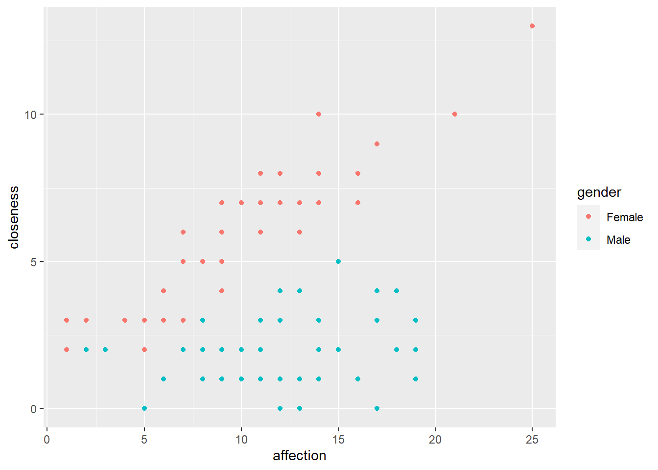
此資料測量觀察到的寵物鸚鵡與其主人的親近度(closeness)、主人表現出的情感行為量(affection)與鸚鵡的性別。
設定工作目錄。
讀入資料。
cData <- read.table("moderation.csv", header=TRUE, sep=",")| affection | closeness | gender_dummy | gender |
|---|---|---|---|
| 7 | 2 | 0 | Male |
| 6 | 1 | 0 | Male |
| 12 | 0 | 0 | Male |
| 14 | 1 | 0 | Male |
| 17 | 3 | 0 | Male |
| 19 | 2 | 0 | Male |
畫情感行為量與親近度的散佈圖,並依據不同的鸚鵡性別上色。
8.2 調節變項為類別變項
以下檢驗是否鸚鵡的性別可以調節主人表現出的情感對他們和鸚鵡之間的親密度。欲測試的想法為:主人表現出的情感對他們和鸚鵡之間的親密度有正向的效果;但對於雄性或雌性鸚鵡,這種效果可能會有所不同。意即,情感對親近的影響是由鸚鵡的性別調節的。
8.2.1 模型檢驗
將情感中心化後,以pequod套件中的lmres()函數做迴歸分析。此函數可直接以type=nested來看兩階段的迴歸模型,一為沒有交互作用項的,一為有交互作用項的,並檢驗加入交互作用項的模型是否顯著。
library(pequod)
m1 <- lmres(closeness~affection*gender, centered=c("affection"), data=cData)
summary(m1, type="nested")
## **Models**
##
## Model 1: closeness ~ affection + genderMale
## <environment: 0x0000021973996168>
##
## Model 2: closeness ~ affection + genderMale + affection.XX.genderMale
## <environment: 0x0000021973996168>
##
##
## **Statistics**
##
## R R^2 Adj. R^2 Diff.R^2 F df1 df2 p.value
## Model 1 0.88 0.77 0.76 0.77 160.04 2.00 97 < 2.2e-16 ***
## Model 2: 0.93 0.86 0.86 0.09 197.52 3.00 96 < 2.2e-16 ***
## ---
## Signif. codes: 0 '***' 0.001 '**' 0.01 '*' 0.05 '.' 0.1 ' ' 1
##
##
## **F change**
##
## Res.Df RSS Df Sum of Sq F Pr(>F)
## 1 97 177
## 2 96 106 1 71 64.1 2.7e-12 ***
## ---
## Signif. codes: 0 '***' 0.001 '**' 0.01 '*' 0.05 '.' 0.1 ' ' 1
##
##
## **Coefficients**
##
## Estimate StdErr t.value beta p.value
## -- Model 1 --
##
## (Intercept) 6.29135 0.19168 32.82144 < 2.2e-16 ***
## affection 0.26269 0.02963 8.86462 0.4367 < 2.2e-16 ***
## genderMale -4.46269 0.27189 -16.41354 -0.8085 < 2.2e-16 ***
##
##
## -- Model 2 --
##
## (Intercept) 6.36873 0.14950 42.60126 < 2.2e-16 ***
## affection 0.41746 0.03009 13.87403 0.6939 < 2.2e-16 ***
## genderMale -4.42985 0.21165 -20.93042 -0.8026 < 2.2e-16 ***
## affection.XX.genderMale -0.37521 0.04685 -8.00877 -0.3996 < 2.2e-16 ***
## ---
## Signif. codes: 0 '***' 0.001 '**' 0.01 '*' 0.05 '.' 0.1 ' ' 1由上面結果可知兩模型皆顯著,但加入交互作用的模型比未加入的模型可以多解釋9%的變異量,此增加的解釋量達到顯著,\(\Delta\)R^2 = .09, F(1,96) = 64.1, p < .001。迴歸式為closeness = 6.37 + 0.42 affection - 4.43 genderM - 0.38 affection\(\times\)genderM。
8.2.2 Simple slope分析
交互作用顯著,表示有調節效果。接著可做Simple slope分析,看鸚鵡的性別為雄性/雌性與情感在正/負一個標準差時的親密程度預測值。
Sim_m1 <- simpleSlope(m1, pred="affection", mod1="genderMale", coded="genderMale")
summary(Sim_m1)
##
## ** Estimated points of closeness **
##
## Low affection (-1 SD) High affection (+1 SD)
## Low genderMale ( 0 ) 4.4440 8.2935
## High genderMale ( 1 ) 1.7441 2.1337
##
##
##
## ** Simple Slopes analysis ( df= 96 ) **
##
## simple slope standard error t-value p.value
## Low genderMale ( 0 ) 0.4175 0.0301 13.87 <2e-16 ***
## High genderMale ( 1 ) 0.0422 0.0359 1.18 0.24
## ---
## Signif. codes: 0 '***' 0.001 '**' 0.01 '*' 0.05 '.' 0.1 ' ' 1
##
##
##
## ** Bauer & Curran 95% CI **
##
## lower CI upper CI
## genderMale 0.9366 1.3778對上述Simple Slope作圖。
PlotSlope(Sim_m1)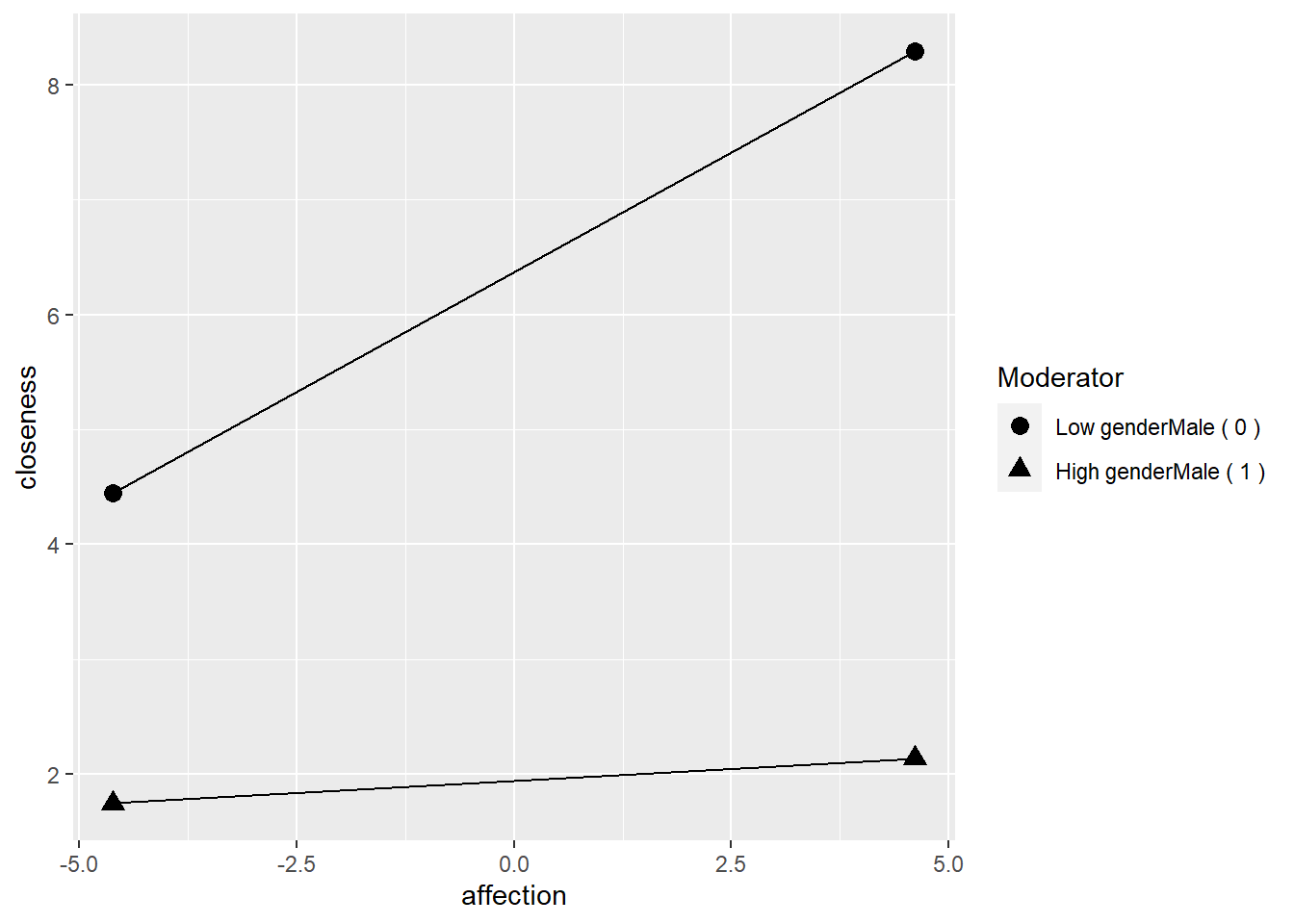
8.3 調節變項為連續變項
8.3.1 模型檢驗
資料與上面相同,但將情感作為調節變項、鸚鵡的性別做為預測項。迴歸式相同,故迴歸分析結果同上。
library(pequod)
m2 <- lmres(closeness~gender*affection, centered=c("affection"), data=cData)
summary(m2, type="nested")
## **Models**
##
## Model 1: closeness ~ genderMale + affection
## <environment: 0x000002197415b570>
##
## Model 2: closeness ~ genderMale + affection + genderMale.XX.affection
## <environment: 0x000002197415b570>
##
##
## **Statistics**
##
## R R^2 Adj. R^2 Diff.R^2 F df1 df2 p.value
## Model 1 0.88 0.77 0.76 0.77 160.04 2.00 97 < 2.2e-16 ***
## Model 2: 0.93 0.86 0.86 0.09 197.52 3.00 96 < 2.2e-16 ***
## ---
## Signif. codes: 0 '***' 0.001 '**' 0.01 '*' 0.05 '.' 0.1 ' ' 1
##
##
## **F change**
##
## Res.Df RSS Df Sum of Sq F Pr(>F)
## 1 97 177
## 2 96 106 1 71 64.1 2.7e-12 ***
## ---
## Signif. codes: 0 '***' 0.001 '**' 0.01 '*' 0.05 '.' 0.1 ' ' 1
##
##
## **Coefficients**
##
## Estimate StdErr t.value beta p.value
## -- Model 1 --
##
## (Intercept) 6.29135 0.19168 32.82144 < 2.2e-16 ***
## genderMale -4.46269 0.27189 -16.41354 -0.8085 < 2.2e-16 ***
## affection 0.26269 0.02963 8.86462 0.4367 < 2.2e-16 ***
##
##
## -- Model 2 --
##
## (Intercept) 6.36873 0.14950 42.60126 < 2.2e-16 ***
## genderMale -4.42985 0.21165 -20.93042 -0.8026 < 2.2e-16 ***
## affection 0.41746 0.03009 13.87403 0.6939 < 2.2e-16 ***
## genderMale.XX.affection -0.37521 0.04685 -8.00877 -0.3996 < 2.2e-16 ***
## ---
## Signif. codes: 0 '***' 0.001 '**' 0.01 '*' 0.05 '.' 0.1 ' ' 18.3.2 Simple slope分析
因交互作用顯著,有調節效果,故同樣做simple slope分析。
Sim_m2 <- simpleSlope(m1, pred="genderMale", mod1="affection", coded="genderMale")
summary(Sim_m2)
##
## ** Estimated points of closeness **
##
## Low genderMale ( 0 ) High genderMale ( 1 )
## Low affection (-1 SD) 4.4440 1.7441
## High affection (+1 SD) 8.2935 2.1337
##
##
##
## ** Simple Slopes analysis ( df= 96 ) **
##
## simple slope standard error t-value p.value
## Low affection (-1 SD) -2.700 0.305 -8.84 <2e-16 ***
## High affection (+1 SD) -6.160 0.300 -20.57 <2e-16 ***
## ---
## Signif. codes: 0 '***' 0.001 '**' 0.01 '*' 0.05 '.' 0.1 ' ' 1
##
##
##
## ** Bauer & Curran 95% CI **
##
## lower CI upper CI
## affection -15.864 -9.2647Simple slope分析結果圖。
PlotSlope(Sim_m2)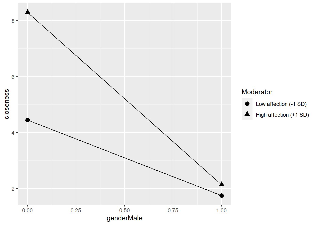
8.3.3 以Johnson-Neyman technique
若要以Johnson-Neyman (JN) technique進一步探究調節效果,需要用R內建的lm()函數來做迴歸。
為了和上面結果相呼應,先產生一個dummy variable: genderD,將男生設為1、女生為0。這邊直接將原dataframe中的gender_dummy以1去減即可。
cData$genderD <- 1 - cData$gender_dummy若資料中沒有gender_dummy變項,也可以用plyr套件中的revalue()函數將Male轉為1、Female轉為0,再用as.numeric()函數將之轉為數值。
library(plyr)
cData$D <- as.numeric(revalue(cData$gender, c("Male"=1, 'Female'=0)))
將情感(affection)中心化,產生一新的變項affectionC。
以affectionC和genderD來預測closeness。
##
## Call:
## lm(formula = closeness ~ affectionC + genderD, data = cData)
##
## Residuals:
##     Min      1Q  Median      3Q     Max
## -3.3733 -0.8598  0.2029  0.8282  3.0625
##
## Coefficients:
##             Estimate Std. Error t value Pr(>|t|)
## (Intercept)  6.29135    0.19168  32.821  < 2e-16 ***
## affectionC   0.26269    0.02963   8.865 3.78e-14 ***
## genderD     -4.46269    0.27189 -16.414  < 2e-16 ***
## ---
## Signif. codes:  0 '***' 0.001 '**' 0.01 '*' 0.05 '.' 0.1 ' ' 1
##
## Residual standard error: 1.351 on 97 degrees of freedom
## Multiple R-squared:  0.7674, Adjusted R-squared:  0.7626
## F-statistic:   160 on 2 and 97 DF,  p-value: < 2.2e-16
上述迴歸式加入affectionC*genderD來預測closeness。
##
## Call:
## lm(formula = closeness ~ affectionC + genderD + affectionC *
##     genderD, data = cData)
##
## Residuals:
##      Min       1Q   Median       3Q      Max
## -2.18730 -0.74369 -0.06341  0.68137  2.89720
##
## Coefficients:
##                    Estimate Std. Error t value Pr(>|t|)
## (Intercept)         6.36873    0.14950  42.601  < 2e-16 ***
## affectionC          0.41746    0.03009  13.874  < 2e-16 ***
## genderD            -4.42985    0.21165 -20.930  < 2e-16 ***
## affectionC:genderD -0.37521    0.04685  -8.009 2.72e-12 ***
## ---
## Signif. codes:  0 '***' 0.001 '**' 0.01 '*' 0.05 '.' 0.1 ' ' 1
##
## Residual standard error: 1.052 on 96 degrees of freedom
## Multiple R-squared:  0.8606, Adjusted R-squared:  0.8562
## F-statistic: 197.5 on 3 and 96 DF,  p-value: < 2.2e-16
以anova()比較兩模型。結果同上,有交互作用項的模型有顯著提高解釋力。
anova(res0, res1)## Analysis of Variance Table
##
## Model 1: closeness ~ affectionC + genderD
## Model 2: closeness ~ affectionC + genderD + affectionC * genderD
## Res.Df RSS Df Sum of Sq F Pr(>F)
## 1 97 177.14
## 2 96 106.19 1 70.948 64.14 2.722e-12 ***
## ---
## Signif. codes: 0 '***' 0.001 '**' 0.01 '*' 0.05 '.' 0.1 ' ' 1用processR來做分析。processR目前無法用在最新版的R 4.2.0版,會讓整個R當掉。但R 4.2.0之前的版本沒有問題。
尤其processR在R 4.2.0會有問題,下面的程式碼請自行執行,不再demo。
用modelSummary()來整理迴歸的結果表。
library(processR)
modelsSummary(res1)
用modelSummary2()來看不同affection(-1SD、0、+1SD)和gender(0、1)組合的closeness。
modSummary2(res1, rangemode=1)用modSummary3()來看conditional effect。結果顯示,當affectionC為0時,slope為-4.43;affectionC為+1 SD時,slope為-2.70;affectionC為-1 SD時,slope為-6.16。
modSummary3(res1, X='genderD', W='affectionC', rangemode=1)8.3.3.1 以rockchalk套件分析
以rockchalk套件的plotSlopes()來畫上述conditional effect的圖。
library(rockchalk)
ps <- plotSlopes(res1, plotx="genderD", modx="affectionC", modxVals="std.dev")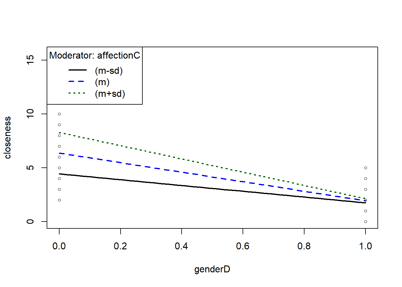
Johnson-Neyman (JN) technique: 檢驗各affectC下的conditional effect,其slope是否顯著。
ts <- testSlopes(ps)## Values of affectionC OUTSIDE this interval:
## lo hi
## -15.931548 -9.238178
## cause the slope of (b1 + b2*affectionC)genderD to be statistically significant
plot(ts)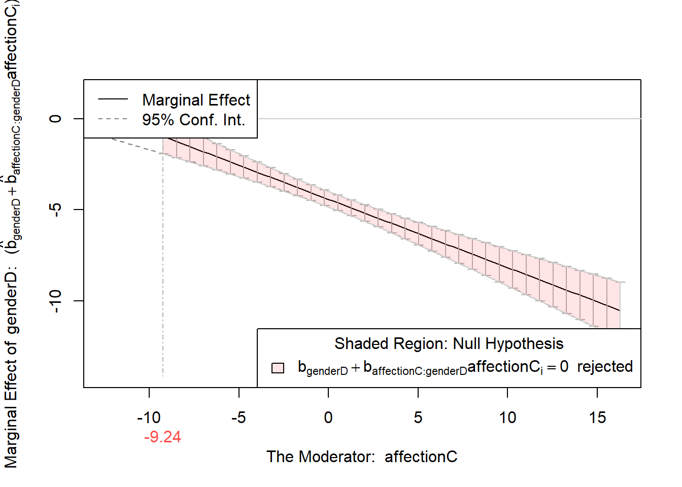
8.3.3.2 以interacions套件分析
interactions套件也提供很好的視覺化圖表功能,可用來看conditional effect與Johnson-Neyman分析。
畫conditional effect的圖,含資料點。
library(interactions)
interact_plot(res1, pred = genderD, modx = affectionC, plot.points = TRUE)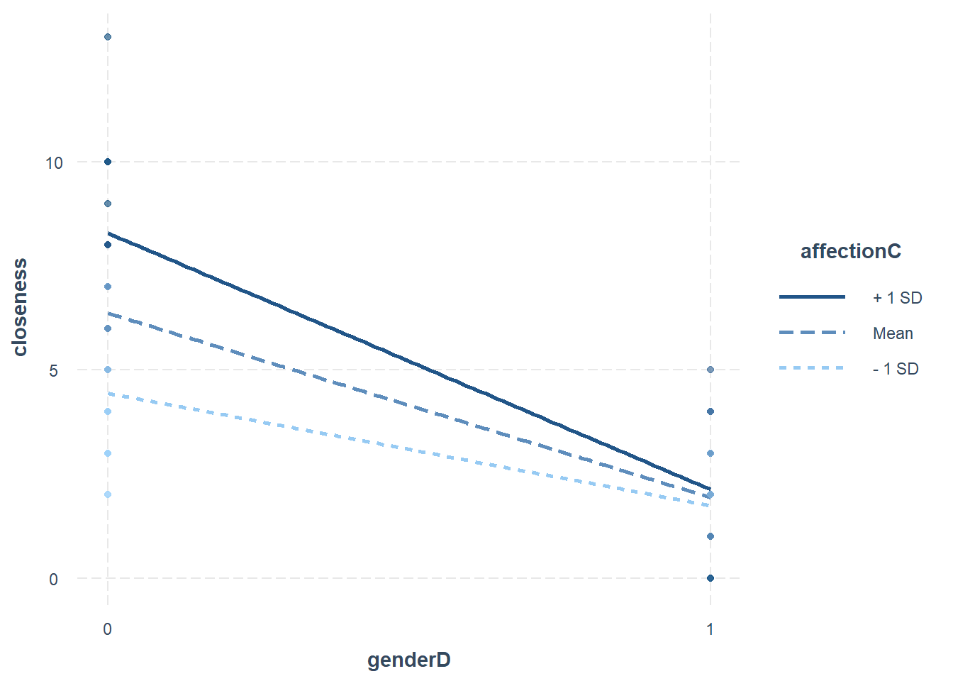
畫conditional effect的圖,含信賴區間。
interact_plot(res1, pred = genderD, modx = affectionC, interval = TRUE)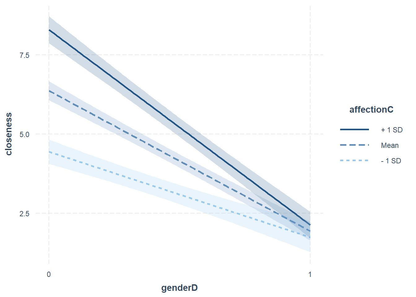
做Johnson-Neyman分析。
sim_slopes(res1, pred = genderD, modx = affectionC, jnplot = TRUE)## JOHNSON-NEYMAN INTERVAL
##
## When affectionC is OUTSIDE the interval [-15.93, -9.24], the slope of
## genderD is p < .05.
##
## Note: The range of observed values of affectionC is [-10.12, 13.88]
## SIMPLE SLOPES ANALYSIS
##
## Slope of genderD when affectionC = -4.61066e+00 (- 1 SD):
##
##    Est.   S.E.   t val.      p
## ------- ------ -------- ------
##   -2.70   0.31    -8.84   0.00
##
## Slope of genderD when affectionC =  7.81597e-16 (Mean):
##
##    Est.   S.E.   t val.      p
## ------- ------ -------- ------
##   -4.43   0.21   -20.93   0.00
##
## Slope of genderD when affectionC =  4.61066e+00 (+ 1 SD):
##
##    Est.   S.E.   t val.      p
## ------- ------ -------- ------
##   -6.16   0.30   -20.57   0.00
或是用john_neyman()函數來做圖。
johnson_neyman(model = res1, pred = genderD, modx = affectionC)## JOHNSON-NEYMAN INTERVAL
##
## When affectionC is OUTSIDE the interval [-15.93, -9.24], the slope of
## genderD is p < .05.
##
## Note: The range of observed values of affectionC is [-10.12, 13.88]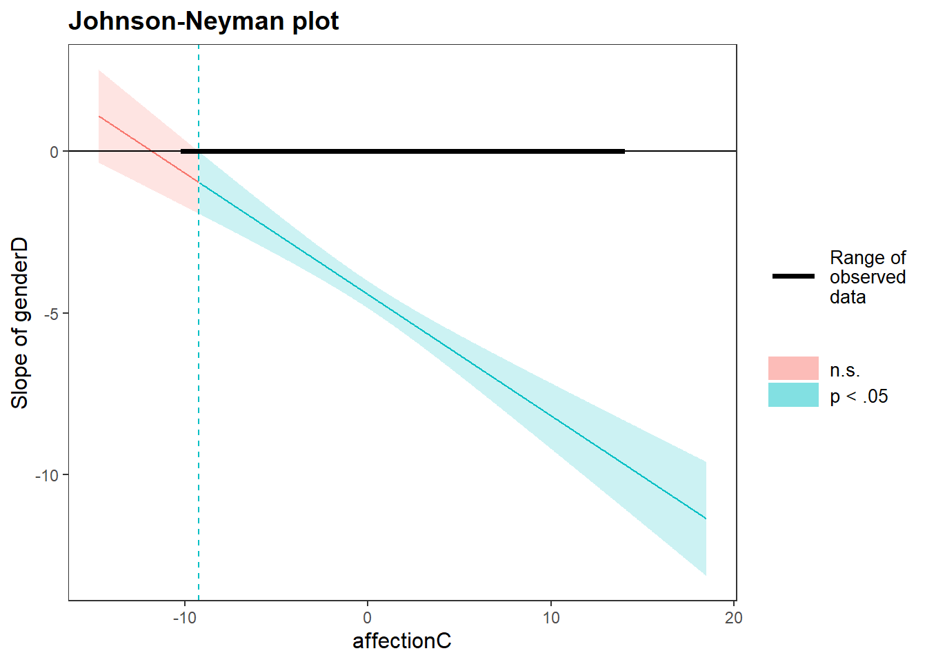
8.3.3.3 用process macro來分析
若是習慣使用Andrew Hayes發展的process macro,可先到process的網站下載檔案。解壓縮後直接執行process.R。可用source(‘檔案路徑’)來執行,或全選後按run執行,前者會快一些,因為不會列印出一堆文字。
source('D:\\Dropbox\\processR\\PROCESS v4.1 for R\\process.R')同上的model,以process來做分析。model=1是調節模型,jn=1表示要執行Johnson–Neyman Technique分析。center=2表示僅將連續變項中心化,plot=1表示要輸出Data for visualizing the conditional effect of the focal predictor。
process(data=cData,y="closeness",x="genderD",w="affection", model=1, center=2, jn=1, plot=1)