第 93 章 Prospensity Score 傾向性評分
Definition 93.1 傾向性評分 propensity score: 如果研究中結果變量為 \(Y\),二分類的暴露變量 \(X\),以及條件變量 \(\mathbf{C}\),那麼每個觀察對象的傾向性評分 \(p\mathbf{C}\) 可以被定義為,一個觀察對象真實被觀察到暴露變量 \(X=1\) 的條件概率(\(p\mathbf{C}\) is defined as the conditional probability of being exposed given covariates):
\[ p(\mathbf{C}) = \text{Pr}(X=1 | \mathbf{C}) \]注意,傾向性評分 propensity score,本質上僅僅只是一個標量 scalar,而不是條件變量那樣的多維變量。
而且,條件可置換性這一重要的前提假設,被 (Rosenbaum and Rubin 1983) 證明是可以拓展到這個標量的:
Theorem 93.1 傾向性評分的最重要性質:
\[ Y(x) \perp\perp X|\mathbf{C}, x=0,1 \Rightarrow Y(x) \perp\perp X|p(\mathbf{C}, x=0, 1) \]
(Rosenbaum and Rubin 1983)這一重要的性質告訴我們,其實在考慮調整混雜因素的時候,我們可以專注考慮這一個標量作爲混雜因素。實際操作中,這個標量通常需要通過一個邏輯回歸模型來擬合計算。這個計算傾向性評分的邏輯回歸模型,用的是對象是否被暴露作爲結果變量,用其他的和這個暴露相關的混雜因素作爲預測變量 \(X|\mathbf{C}\)。
93.0.1 關於條件可置換性
如果兩個觀察對象,經過計算,他們二人的傾向性評分相同,那麼從這些條件變量來看,這兩個對象是否被暴露,就是完全隨機的,他們有相同的概率屬於被暴露或非暴露人羣。這一點和RCT有些相似,如果,一個完美的隨機化試驗,那麼一個患者被分進治療組或者對照組的概率是完全相同的,他們是完全可以置換的 (exchangeable)。所以,在一個觀察性研究中,如果傾向性評分相同,在給定的觀察到的所有混雜因素的條件下,這兩個對象是否暴露的概率是相同的 (可以條件置換的 conditional exchangeability given the propensity score)。
當然和RCT相比,這兩個概念的本質區別在於,隨機化臨牀實驗是通過實驗設計手段,保證了研究對象的完全可置換。觀察性研究,則沒有這個優點,因爲他們的可置換性質是由觀察到的混雜因子決定的,許多觀察性研究的混雜因子都無法保證全部觀察得到。條件可置換性是一個非常強的假設,因爲它假定我們真的把所有的混雜都觀察到了。
這個例子中的混雜因子包括: 年齡,性別,醫院 (1/2/3/4),吸煙 (non, ex, current),腫塊數量,其他腫瘤轉移部位,患者已患癌症的時間,腫塊的大小,主要癌症的部位 (膀胱,乳腺,大腸,食道,腎,皮膚,胃,睾丸等),還有一個腫塊是否容易被摘除的難易程度 (容易,中等,困難)。那麼,我們可以給患者擬合下面的模型做傾向性評分:
\[ \begin{aligned} \text{logit}\{ \text{Pr(RFA}|\mathbf{C} \} = & \beta_0 + \beta_1\text{age} + \beta_2 \text{gender}+ \beta_3I(\text{hospital = 2}) \\ & +\beta_4I(\text{hospital =3}) + \beta_5I(\text{hospital = 4}) + \beta_6I(\text{smoke = 2} )\\ & + \beta_7I(\text{smoke = 3}) + \beta_8\text{nodules} + \beta_9\text{mets} + \beta_{10}\text{duration} \\ & + \cdots + \beta_{20}I(\text{primary = 9}) + \beta_{21}I(\text{position = 2}) + \beta_{22}I(\text{position = 3}) \end{aligned} \]
擬合了這個模型,計算每個參數 \(\beta_0 sim \beta_22\) 的極大似然估計之後,就可以計算每個患者的傾向性評分:
\[ \begin{aligned} \hat{p}(\mathbf{C}_i) = & \text{expit}\{ \hat\beta_0 + \hat\beta_1\text{age} + \hat\beta_2 \text{gender}+ \hat\beta_3I(\text{hospital = 2}) \\ & +\hat\beta_4I(\text{hospital =3}) + \hat\beta_5I(\text{hospital = 4}) + \hat\beta_6I(\text{smoke = 2} )\\ & + \hat\beta_7I(\text{smoke = 3}) + \hat\beta_8\text{nodules} + \hat\beta_9\text{mets} + \hat\beta_{10}\text{duration} \\ & + \cdots + \hat\beta_{20}I(\text{primary = 9}) + \hat\beta_{21}I(\text{position = 2}) + \hat\beta_{22}I(\text{position = 3}) \} \end{aligned} \]
其中
\[ \text{expit}(a) = \frac{\exp(a)}{1+\exp(a)} \]
下面就是傾向性評分模型的輸出結果:
##
## Call:
## glm(formula = rfa ~ age + gender + smoke + hospital + nodules +
##     mets + duration + maxdia + primary + position, family = binomial(link = logit),
##     data = RFAcat)
##
## Deviance Residuals:
##      Min        1Q    Median        3Q       Max
## -2.53460  -0.86875  -0.30119   0.89717   2.64611
##
## Coefficients:
##                Estimate  Std. Error  z value  Pr(>|z|)
## (Intercept)  2.95798757  0.61770661   4.7887 1.679e-06 ***
## age         -0.00044027  0.00992941  -0.0443   0.96463
## gender1      0.10435375  0.15103436   0.6909   0.48961
## smoke1       0.11861648  0.15106839   0.7852   0.43235
## smoke2       0.09342271  0.10380671   0.9000   0.36814
## hospital2   -0.23564078  0.14243617  -1.6544   0.09805 .
## hospital3    0.30045787  0.13850888   2.1692   0.03007 *
## hospital4   -0.11174925  0.19236619  -0.5809   0.56129
## nodules     -0.02987712  0.01820608  -1.6411   0.10079
## mets         0.06514394  0.04672394   1.3942   0.16325
## duration     0.00260668  0.00488559   0.5335   0.59366
## maxdia      -2.26045488  0.08773789 -25.7637 < 2.2e-16 ***
## primary2     0.09927913  0.29102032   0.3411   0.73300
## primary3     0.14593436  0.29460236   0.4954   0.62035
## primary4    -0.00212669  0.38021005  -0.0056   0.99554
## primary5    -0.22135219  0.37933124  -0.5835   0.55953
## primary6     0.04504894  0.34609342   0.1302   0.89644
## primary7     1.57439087  0.64792618   2.4299   0.01510 *
## primary8     0.21261200  0.38272919   0.5555   0.57854
## primary9     0.33223472  0.40566455   0.8190   0.41279
## position2    0.94096446  0.10080061   9.3349 < 2.2e-16 ***
## position3    1.22134526  0.11678128  10.4584 < 2.2e-16 ***
## ---
## Signif. codes:  0 '***' 0.001 '**' 0.01 '*' 0.05 '.' 0.1 ' ' 1
##
## (Dispersion parameter for binomial family taken to be 1)
##
##     Null deviance: 4916.81  on 3550  degrees of freedom
## Residual deviance: 3834.74  on 3529  degrees of freedom
## AIC: 3878.74
##
## Number of Fisher Scoring iterations: 4
正如我們預料的那樣,醫院,腫塊尺寸,和腫塊的位置是患者接受 RFA 治療與否的重要預測指標。
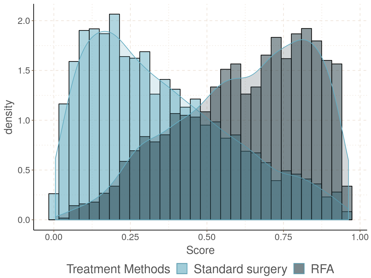
圖 93.1: Density and histogram of the estimated propensity score in the two exposure groups.
從圖 93.1 可以看出評分在兩個暴露組中的分布交叉十分令人滿意。
93.1 怎樣使用傾向性評分
傾向性評分在實際操作中的運用:
- 分層 stratification: 把觀察對象按照傾向性評分的高低分層成爲幾個組,進行組內的療效比較;
- 配對 matching: 在真實的暴露組中的對象,爲他們每個人找一個非暴露的人,一兩個對象的傾向性評分盡可能接近爲配對的方法;
- 在模型中調整 adjustment: 在回歸模型中調整這個傾向性評分,而不是調整那些計算評分時的那些條件變量;
- 給每個研究對象按照其評分得分,使用逆向加權法 (inverse weighting)。
93.1.1 分層法 stratification
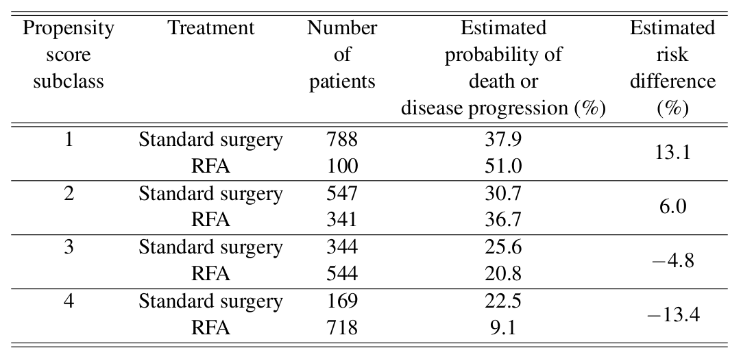
\[ \widehat{\text{ACE}} = \frac{13.1 + 6.0 - 4.8 - 13.4}{4} = 0.2% \]
\[ \begin{aligned} \widehat{\text{ATT}} & = \frac{13.1\times100 + 6.0\times341 - 4.8\times544 - 13.4\times718}{100 + 341 + 544 + 718} \\ & = -5.2%\\ \end{aligned} \]
再次印證了之前一章練習中的計算結果,也就是 RFA 如果施加給整體患者,那麼甚至可能還稍微提高三年內死亡/病情加重的概率。但是如果只給適合 RFA 療法的人,那麼 RFA 能明顯地降低死亡/病情加重的概率。
93.1.2 配對法 matching
用肺癌數據的例子來解釋,就是
從選擇了 RFA 療法的患者出發,在標準療法的患者中尋找一名或者多名和 RFA 療法患者的評分接近的患者作對照,這樣計算的是 ATT (average treatment effect in the treated)。
從選擇了標準手術療法的患者出發,在 RFA 療法的患者中尋找一名或者多名和 RFA 療法患者的評分接近的患者作對照,這樣計算的是 非暴露組中的平均療效 (average treatment effect in the untreated/unexposed)。
此時,配對患者選用是可以重復出現的 (replacement is allowed),所以,有的對照可能同時給好幾個病例做對照也有可能。所以當你的樣本可能不平衡,那麼從樣本量大的那一部分出發的時候,就會出現這種情況。
選擇配對的方法也有很多:
- nearest neighbour matching (wthin calipers defined by the PS)
- Kernel matching (nearest neighbour matching chooses one match)
- etc.
如果數據不適合使用傾向性評分法,那麼只要一做配對,就能立刻發現數據的問題,因爲如果違反了 positivity,那麼樣本中的某一組患者可能就大量地找不到相同相似PS評分的配對。另外配對法,可以配合調整變量共同使用,以增加估計的效能和穩健性。從經驗上來看 1:1 配對常常造成的效果是統計效能較低,而且即使使用配對法,觀察性研究還是觀察性研究,殘差混雜 (residual confounding) 依然存在。而且配對法導致估計量的標準誤難以估計,即使用自助重抽 (bootstrapping) 也常常是沒有效果。還好牛人 (Abadie and Imbens 2016) 發現並發表了配對評分時的有效方差估計法,這個方法也已經加入了 STATA。
在 STATA 裏使用 teffects psmatch 命令執行傾向性評分的配對法
##
## . use "backupfiles/RFA.dta"
##
## . teffects psmatch (dodp) (rfa age gender i.smoke i.hospital nodules mets durat
## > ion maxdia i.primary i.position, logit)
##
## Treatment-effects estimation                   Number of obs      =      3,551
## Estimator      : propensity-score matching     Matches: requested =          1
## Outcome model  : matching                                     min =          1
## Treatment model: logit                                        max =          1
## ------------------------------------------------------------------------------
##              |              AI Robust
##         dodp |      Coef.   Std. Err.      z    P>|z|     [95% Conf. Interval]
## -------------+----------------------------------------------------------------
## ATE          |
##          rfa |
## (radiofre..  |
##          vs  |
## standard..)  |   .0154886   .0204308     0.76   0.448     -.024555    .0555322
## ------------------------------------------------------------------------------
##
## .
## . teffects psmatch (dodp) (rfa age gender i.smoke i.hospital nodules mets durat
## > ion maxdia i.primary i.position, logit), atet
##
## Treatment-effects estimation                   Number of obs      =      3,551
## Estimator      : propensity-score matching     Matches: requested =          1
## Outcome model  : matching                                     min =          1
## Treatment model: logit                                        max =          1
## ------------------------------------------------------------------------------
##              |              AI Robust
##         dodp |      Coef.   Std. Err.      z    P>|z|     [95% Conf. Interval]
## -------------+----------------------------------------------------------------
## ATET         |
##          rfa |
## (radiofre..  |
##          vs  |
## standard..)  |  -.0387551   .0199095    -1.95   0.052    -.0777771    .0002668
## ------------------------------------------------------------------------------
可見,結果和目前爲止計算的結果是吻合的。值得注意的是,配對法在文獻中被發現是最常(濫)用的方法,這裏提評分的配對法,不是因爲我贊成使用這種方法,而是因爲它常見,所以你需要知道這種配對的背後到底在幹啥。顯而易見的是,傾向性評分有它更好的使用方法 (逆向權重)。
93.1.3 回歸模型校正法 adjustment
\[ E\{Y|X,p(\mathbf{C}) \} = \alpha + \beta X + \gamma p(\mathbf{C}) \]
校正傾向性評分,可以一定程度上克服有限樣本造成的偏倚 (finite sample bias)。
93.2 Practical05 - causal inference
數據還是和前一章節一樣的數據。傾向性評分的 R 包有很多,下面用 R 來進行大多數的計算。
93.2.1 初步熟悉數據內容
##
## . use "backupfiles/RFAcat.dta"
##
## . describe
##
## Contains data from backupfiles/RFAcat.dta
##   obs:         3,551
##  vars:            18                          5 Nov 2013 15:05
##  size:       255,672
## -------------------------------------------------------------------------------
##               storage   display    value
## variable name   type    format     label      variable label
## -------------------------------------------------------------------------------
## id              float   %9.0g                 Patient ID
## age             float   %9.0g
## gender          float   %9.0g      gender
## smoke           float   %9.0g      smoke      Smoking status
## hospital        float   %9.0g                 Hospital ID
## nodules         float   %9.0g                 Number of nodules
## mets            float   %9.0g                 Number of other metastatic sites
## duration        float   %9.0g                 Duration of disease (in months)
## maxdia          float   %9.0g                 Diameter of largest nodule (in
##                                                 cm)
## primary         float   %22.0g     primary    Location of primary cancer
## position        float   %9.0g      position   Ease with which nodules can be
##                                                 reached
## coag            float   %9.0g      coag       Coagulopathy
## rfa             float   %23.0g     rfa        Treatment variable: RFA or
##                                                 standard surgery
## dodp            float   %9.0g      dodp       Outcome variable: death or
##                                                 disease progression within 36
##                                                 months
## agecat          float   %9.0g      agecat     Age in categories
## nodcat          float   %9.0g      nodcat     Number of nodules in categories
## durcat          float   %12.0g     durcat     Duration of disease in categories
## diacat          float   %9.0g      diacat     Diameter of largest nodule in
##                                                 categories
## -------------------------------------------------------------------------------
## Sorted by: id
##
## .
## . **********************
## . *  Explore the data  *
## . **********************
## .
## . /*  Question 1  */
## . * Exposure and outcome
## . tab rfa
##
## Treatment variable: RFA |
##     or standard surgery |      Freq.     Percent        Cum.
## ------------------------+-----------------------------------
##        standard surgery |      1,848       52.04       52.04
## radiofrequency ablation |      1,703       47.96      100.00
## ------------------------+-----------------------------------
##                   Total |      3,551      100.00
##
## . tab dodp rfa, col
##
## +-------------------+
## | Key               |
## |-------------------|
## |     frequency     |
## | column percentage |
## +-------------------+
##
##    Outcome |
##  variable: |
##   death or |
##    disease |  Treatment variable:
## progressio |    RFA or standard
##   n within |        surgery
##  36 months | standard   radiofreq |     Total
## -----------+----------------------+----------
##         no |     1,255      1,349 |     2,604
##            |     67.91      79.21 |     73.33
## -----------+----------------------+----------
##        yes |       593        354 |       947
##            |     32.09      20.79 |     26.67
## -----------+----------------------+----------
##      Total |     1,848      1,703 |     3,551
##            |    100.00     100.00 |    100..
## . * New (categorised) variables:
## . tab1 agecat nodcat durcat diacat, m
##
## -> tabulation of agecat
##
##      Age in |
##  categories |      Freq.     Percent        Cum.
## ------------+-----------------------------------
##         <45 |         96        2.70        2.70
##       45-49 |        860       24.22       26.92
##       50-54 |      1,755       49.42       76.34
##       55-59 |        662       18.64       94.99
##       60-64 |        135        3.80       98.79
##         65+ |         43        1.21      100.00
## ------------+-----------------------------------
##       Total |      3,551      100.00
##
## -> tabulation of nodcat
##
##   Number of |
##  nodules in |
##  categories |      Freq.     Percent        Cum.
## ------------+-----------------------------------
##           1 |        997       28.08       28.08
##           2 |      1,350       38.02       66.09
##           3 |        635       17.88       83.98
##           4 |        204        5.74       89.72
##         5-9 |        304        8.56       98.28
##         10+ |         61        1.72      100.00
## ------------+-----------------------------------
##       Total |      3,551      100.00
##
## -> tabulation of durcat
##
##  Duration of |
##   disease in |
##   categories |      Freq.     Percent        Cum.
## -------------+-----------------------------------
##   <10 months |         53        1.49        1.49
## 10-19 months |      1,437       40.47       41.96
## 20-29 months |      1,528       43.03       84.99
## 30-39 months |        397       11.18       96.17
##   40+ months |        136        3.83      100.00
## -------------+-----------------------------------
##        Total |      3,551      100.00
##
## -> tabulation of diacat
##
## Diameter of |
##     largest |
##   nodule in |
##  categories |      Freq.     Percent        Cum.
## ------------+-----------------------------------
##     <1.5 cm |        967       27.23       27.23
##   1.5-1.9cm |      1,147       32.30       59.53
##     2-2.4cm |        940       26.47       86.00
##   2.5-2.9cm |        403       11.35       97.35
##        3cm+ |         94        2.65      100.00
## ------------+-----------------------------------
##       Total |      3,551      100.00
##
## .
93.2.2 把連續型變量以分類型數據的形式放入模型中:
***************************
*  Regression adjustment  *
***************************

/*  Question 2  */
// teffects ra (dodp   i.agecat gender i.smoke i.hospital i.nodcat ///
// i.mets i.durcat i.diacat i.primary i.position,   ///
// logit) (rfa)
你會發現 STATA 停不下來,計算永遠都不會收斂。這是因爲我們在這個模型中結果部分加入了太多的分類型變量,但數據又沒辦法進行足夠的計算。
93.2.3 用相同的模型結構估計每個人的傾向性評分
RFAcat <- read_dta("backupfiles/RFAcat.dta")
RFAcat <- RFAcat %>%
  mutate(gender = factor(gender, labels = c("men", "women")),
         smoke = factor(smoke, labels = c("never", "ex", "current")),
         hospital = as.factor(hospital),
         primary = factor(primary, labels =  c("bladder",
                                     "breast",
                                     "colorectal",
                                     "gullet",
                                     "kidney",
                                     "prostate",
                                     "skin",
                                     "stomach",
                                     "testicular")),
         position = factor(position, labels = c("easy", "moderate", "difficult")),
         nodcat = factor(nodcat, labels = c("1","2","3","4","5-9","10+")),
         mets = as.factor(mets),
         agecat = factor(agecat, labels = c("< 45", "45-49", "50-54", "55-59", "60-64","65+")),
         durcat = factor(durcat, labels = c("< 10m", "10-19m", "20-29m", "30-39m", "40+m")),
         diacat = factor(diacat, labels = c("<1.5cm", "1.5-1.9cm", "2-2.4cm", "2.5-2.9cm",
                                            "3cm+")))
Pros_Score <- glm(rfa ~ agecat + gender + smoke + hospital + nodcat + mets +
                    durcat + diacat + primary + position, family = binomial(link = logit),
                  data = RFAcat)
summary(Pros_Score)
##
## Call:
## glm(formula = rfa ~ agecat + gender + smoke + hospital + nodcat +
## mets + durcat + diacat + primary + position, family = binomial(link = logit),
## data = RFAcat)
##
## Deviance Residuals:
## Min 1Q Median 3Q Max
## -2.45628 -0.90333 -0.26702 0.90927 2.67426
##
## Coefficients:
## Estimate Std. Error z value Pr(>|z|)
## (Intercept) 0.243514 0.505730 0.4815 0.630154
## agecat45-49 0.090044 0.261908 0.3438 0.730996
## agecat50-54 0.107064 0.255438 0.4191 0.675115
## agecat55-59 -0.040906 0.269042 -0.1520 0.879154
## agecat60-64 0.074712 0.327138 0.2284 0.819351
## agecat65+ 0.398326 0.431966 0.9221 0.356464
## genderwomen 0.083521 0.151596 0.5509 0.581673
## smokeex 0.117319 0.150316 0.7805 0.435105
## smokecurrent 0.144515 0.104757 1.3795 0.167732
## hospital2 -0.190892 0.140877 -1.3550 0.175407
## hospital3 0.345035 0.138004 2.5002 0.012413 *
## hospital4 -0.094451 0.191935 -0.4921 0.622648
## nodcat2 -0.085830 0.097834 -0.8773 0.380324
## nodcat3 -0.012021 0.118491 -0.1014 0.919195
## nodcat4 0.143596 0.182086 0.7886 0.430336
## nodcat5-9 -0.482427 0.156551 -3.0816 0.002059 **
## nodcat10+ 0.043502 0.299620 0.1452 0.884561
## mets1 0.100543 0.099312 1.0124 0.311349
## mets2 0.139866 0.105583 1.3247 0.185272
## mets3 -0.091375 0.296308 -0.3084 0.757795
## durcat10-19m 0.038115 0.342352 0.1113 0.911352
## durcat20-29m -0.009245 0.341993 -0.0270 0.978434
## durcat30-39m 0.127019 0.356684 0.3561 0.721758
## durcat40+m 0.159252 0.394089 0.4041 0.686138
## diacat1.5-1.9cm -1.053938 0.100734 -10.4626 < 2.2e-16 ***
## diacat2-2.4cm -2.223150 0.109874 -20.2337 < 2.2e-16 ***
## diacat2.5-2.9cm -3.781319 0.199920 -18.9142 < 2.2e-16 ***
## diacat3cm+ -4.216794 0.470139 -8.9693 < 2.2e-16 ***
## primarybreast 0.070017 0.288955 0.2423 0.808540
## primarycolorectal 0.087730 0.292264 0.3002 0.764044
## primarygullet -0.091053 0.378701 -0.2404 0.809993
## primarykidney -0.269296 0.377865 -0.7127 0.476046
## primaryprostate -0.027718 0.344383 -0.0805 0.935850
## primaryskin 1.557764 0.670168 2.3244 0.020102 *
## primarystomach 0.134603 0.380885 0.3534 0.723792
## primarytesticular 0.304981 0.403875 0.7551 0.450167
## positionmoderate 0.891048 0.099587 8.9474 < 2.2e-16 ***
## positiondifficult 1.178730 0.116364 10.1296 < 2.2e-16 ***
## ---
## Signif. codes: 0 '***' 0.001 '**' 0.01 '*' 0.05 '.' 0.1 ' ' 1
##
## (Dispersion parameter for binomial family taken to be 1)
##
## Null deviance: 4916.81 on 3550 degrees of freedom
## Residual deviance: 3852.35 on 3513 degrees of freedom
## AIC: 3928.35
##
## Number of Fisher Scoring iterations: 5RFAcat$Score <- Pros_Score$fitted.values # extract the fitted scores
ggthemr('fresh', layout = 'scientific')
RFAcat %>%
ggplot(aes(x = Score, y= ..density.., fill = as.factor(rfa))) +
geom_histogram(position = "identity", color = "black", alpha = 0.5) +
geom_density(alpha = 0.2) +
theme(axis.title = element_text(size = 17), axis.text = element_text(size = 14),
axis.line = element_line(colour = "black"),
panel.border = element_blank(),
panel.background = element_blank()) +
theme(legend.text = element_text(size = 19),
legend.title = element_text(size = 19),
legend.position = "bottom", legend.direction = "horizontal") +
labs(fill = "Treatment Methods") +
scale_fill_discrete(labels = c("Standard surgery", "RFA")); ggthemr_reset()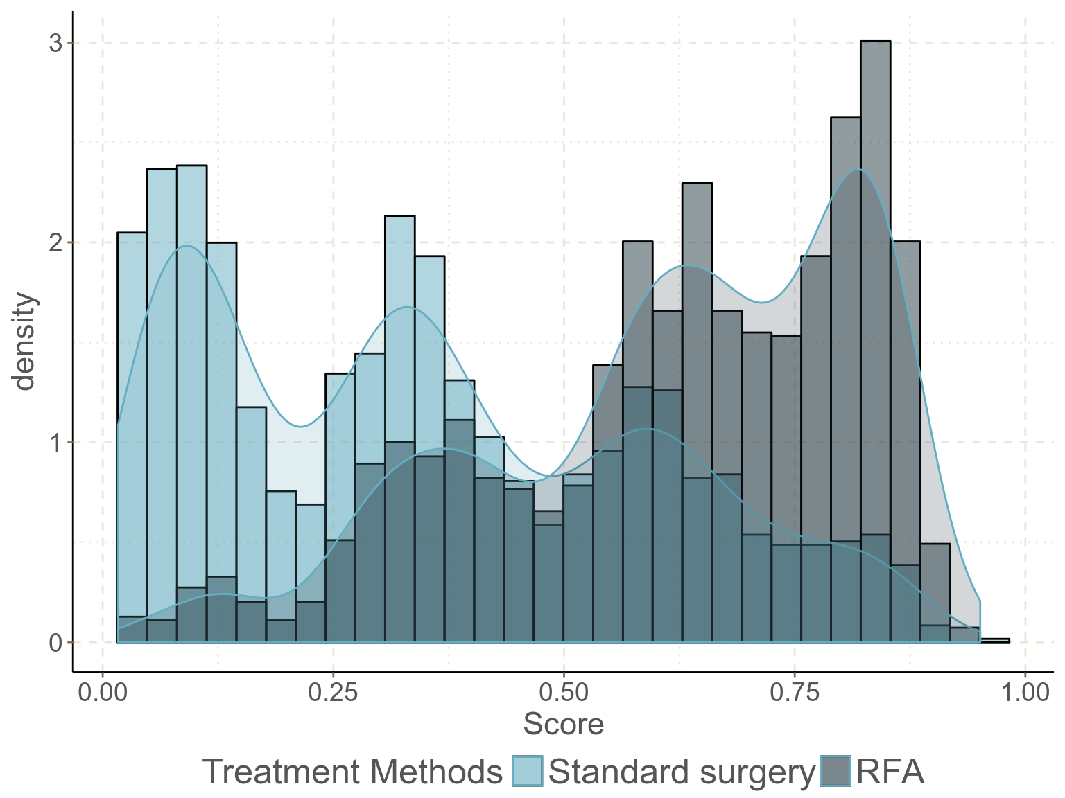
圖 93.2: Density and histogram of the estimated propensity score in the two exposure groups, with confounders and predictors of outcome included in the PS model.
概率密度分布圖和直方圖的內容告訴我們兩個暴露組患者的評分分布的交叉部分十分令人滿意,positivity 的前提假設可認爲得到滿足 (每個患者都有非零的概率接受 RFA 或者標準手術療法)。
一種比較組與組之間不同量的指標: standardized (mean) difference (Austin 2011),可以用下面的方法來計算,使用 tableone 這個方便的 R 包:
# covariates
Cov <- c("agecat", "gender", "smoke", "hospital", "nodcat", "mets", "durcat", "diacat",
         "primary", "position")
## Construct a table
tabUnmatched <- CreateTableOne(vars = Cov, strata = "rfa", data = RFAcat, test = FALSE)
## Show table with SMD
print(tabUnmatched, smd = TRUE)
## Stratified by rfa
## 0 1 SMD
## n 1848 1703
## agecat (%) 0.065
## < 45 51 ( 2.8) 45 ( 2.6)
## 45-49 463 (25.1) 397 (23.3)
## 50-54 891 (48.2) 864 (50.7)
## 55-59 352 (19.0) 310 (18.2)
## 60-64 72 ( 3.9) 63 ( 3.7)
## 65+ 19 ( 1.0) 24 ( 1.4)
## gender = women (%) 726 (39.3) 701 (41.2) 0.038
## smoke (%) 0.031
## never 1279 (69.2) 1157 (67.9)
## ex 135 ( 7.3) 136 ( 8.0)
## current 434 (23.5) 410 (24.1)
## hospital (%) 0.115
## 1 308 (16.7) 262 (15.4)
## 2 349 (18.9) 282 (16.6)
## 3 677 (36.6) 718 (42.2)
## 4 514 (27.8) 441 (25.9)
## nodcat (%) 0.096
## 1 505 (27.3) 492 (28.9)
## 2 703 (38.0) 647 (38.0)
## 3 325 (17.6) 310 (18.2)
## 4 104 ( 5.6) 100 ( 5.9)
## 5-9 181 ( 9.8) 123 ( 7.2)
## 10+ 30 ( 1.6) 31 ( 1.8)
## mets (%) 0.061
## 0 1089 (58.9) 969 (56.9)
## 1 393 (21.3) 375 (22.0)
## 2 327 (17.7) 331 (19.4)
## 3 39 ( 2.1) 28 ( 1.6)
## durcat (%) 0.070
## < 10m 31 ( 1.7) 22 ( 1.3)
## 10-19m 731 (39.6) 706 (41.5)
## 20-29m 820 (44.4) 708 (41.6)
## 30-39m 197 (10.7) 200 (11.7)
## 40+m 69 ( 3.7) 67 ( 3.9)
## diacat (%) 1.086
## <1.5cm 222 (12.0) 745 (43.7)
## 1.5-1.9cm 507 (27.4) 640 (37.6)
## 2-2.4cm 661 (35.8) 279 (16.4)
## 2.5-2.9cm 369 (20.0) 34 ( 2.0)
## 3cm+ 89 ( 4.8) 5 ( 0.3)
## primary (%) 0.126
## bladder 46 ( 2.5) 35 ( 2.1)
## breast 423 (22.9) 401 (23.5)
## colorectal 694 (37.6) 671 (39.4)
## gullet 75 ( 4.1) 55 ( 3.2)
## kidney 66 ( 3.6) 47 ( 2.8)
## prostate 365 (19.8) 324 (19.0)
## skin 5 ( 0.3) 17 ( 1.0)
## stomach 86 ( 4.7) 67 ( 3.9)
## testicular 88 ( 4.8) 86 ( 5.0)
## position (%) 0.332
## easy 565 (30.6) 292 (17.1)
## moderate 899 (48.6) 921 (54.1)
## difficult 384 (20.8) 490 (28.8)## Count covariates with important imbalance
addmargins(table(ExtractSmd(tabUnmatched) > 0.08))##
## FALSE TRUE Sum
## 5 5 10嚴重不平衡的變量有 5 個: hospital, nodcat, diaact, primary, position。
93.2.4 用 PS 評分來把對象分層 stratification
RFAcat <- RFAcat %>%
  mutate(psblock = ntile(Score, 4))

RFAcat %>%
  group_by(psblock) %>%
    summarise(n(), min(Score), max(Score))
## # A tibble: 4 x 4
## psblock `n()` `min(Score)` `max(Score)`
## <int> <int> <dbl> <dbl>
## 1 1 888 0.0167 0.280
## 2 2 888 0.281 0.508
## 3 3 888 0.508 0.695
## 4 4 887 0.696 0.951但是你看每層的傾向性評分其實範圍有點寬,提示使用分層的方法可能殘餘的混雜有點多。
看每層內數據的平衡:
# Cov <- c("diacat", "position")
#---------------------------------------------#
#  in strata == 1                             #
#                                             #
#---------------------------------------------#
## Construct a table
tabUnmatched <- CreateTableOne(vars = Cov, strata = "rfa", data = RFAcat[RFAcat$psblock == 1,], test = FALSE)
## Show table with SMD
print(tabUnmatched, smd = TRUE)
## Stratified by rfa
## 0 1 SMD
## n 777 111
## agecat (%) 0.321
## < 45 27 ( 3.5) 3 ( 2.7)
## 45-49 211 (27.2) 25 (22.5)
## 50-54 334 (43.0) 59 (53.2)
## 55-59 162 (20.8) 23 (20.7)
## 60-64 37 ( 4.8) 1 ( 0.9)
## 65+ 6 ( 0.8) 0 ( 0.0)
## gender = women (%) 304 (39.1) 45 (40.5) 0.029
## smoke (%) 0.248
## never 533 (68.6) 88 (79.3)
## ex 56 ( 7.2) 6 ( 5.4)
## current 188 (24.2) 17 (15.3)
## hospital (%) 0.265
## 1 135 (17.4) 10 ( 9.0)
## 2 152 (19.6) 27 (24.3)
## 3 270 (34.7) 38 (34.2)
## 4 220 (28.3) 36 (32.4)
## nodcat (%) 0.209
## 1 201 (25.9) 24 (21.6)
## 2 293 (37.7) 47 (42.3)
## 3 119 (15.3) 17 (15.3)
## 4 41 ( 5.3) 7 ( 6.3)
## 5-9 112 (14.4) 16 (14.4)
## 10+ 11 ( 1.4) 0 ( 0.0)
## mets (%) 0.141
## 0 463 (59.6) 70 (63.1)
## 1 154 (19.8) 24 (21.6)
## 2 138 (17.8) 15 (13.5)
## 3 22 ( 2.8) 2 ( 1.8)
## durcat (%) 0.209
## < 10m 17 ( 2.2) 3 ( 2.7)
## 10-19m 297 (38.2) 41 (36.9)
## 20-29m 356 (45.8) 54 (48.6)
## 30-39m 76 ( 9.8) 12 (10.8)
## 40+m 31 ( 4.0) 1 ( 0.9)
## diacat (%) 0.515
## <1.5cm 0 ( 0.0) 0 ( 0.0)
## 1.5-1.9cm 9 ( 1.2) 4 ( 3.6)
## 2-2.4cm 310 (39.9) 68 (61.3)
## 2.5-2.9cm 369 (47.5) 34 (30.6)
## 3cm+ 89 (11.5) 5 ( 4.5)
## primary (%) 0.279
## bladder 23 ( 3.0) 1 ( 0.9)
## breast 180 (23.2) 25 (22.5)
## colorectal 273 (35.1) 43 (38.7)
## gullet 40 ( 5.1) 3 ( 2.7)
## kidney 34 ( 4.4) 7 ( 6.3)
## prostate 159 (20.5) 25 (22.5)
## skin 1 ( 0.1) 1 ( 0.9)
## stomach 32 ( 4.1) 3 ( 2.7)
## testicular 35 ( 4.5) 3 ( 2.7)
## position (%) 0.181
## easy 319 (41.1) 36 (32.4)
## moderate 342 (44.0) 55 (49.5)
## difficult 116 (14.9) 20 (18.0)## Count covariates with important imbalance
addmargins(table(ExtractSmd(tabUnmatched) > 0.08))##
## FALSE TRUE Sum
## 1 9 10#---------------------------------------------#
# in strata == 2 #
# #
#---------------------------------------------#
## Construct a table
tabUnmatched <- CreateTableOne(vars = Cov, strata = "rfa", data = RFAcat[RFAcat$psblock == 2,], test = FALSE)
## Show table with SMD
print(tabUnmatched, smd = TRUE)## Stratified by rfa
## 0 1 SMD
## n 550 338
## agecat (%) 0.114
## < 45 12 ( 2.2) 5 ( 1.5)
## 45-49 129 (23.5) 82 (24.3)
## 50-54 294 (53.5) 173 (51.2)
## 55-59 87 (15.8) 61 (18.0)
## 60-64 21 ( 3.8) 10 ( 3.0)
## 65+ 7 ( 1.3) 7 ( 2.1)
## gender = women (%) 217 (39.5) 132 (39.1) 0.008
## smoke (%) 0.091
## never 384 (69.8) 222 (65.7)
## ex 39 ( 7.1) 29 ( 8.6)
## current 127 (23.1) 87 (25.7)
## hospital (%) 0.101
## 1 91 (16.5) 48 (14.2)
## 2 89 (16.2) 49 (14.5)
## 3 226 (41.1) 154 (45.6)
## 4 144 (26.2) 87 (25.7)
## nodcat (%) 0.139
## 1 150 (27.3) 102 (30.2)
## 2 205 (37.3) 124 (36.7)
## 3 117 (21.3) 61 (18.0)
## 4 37 ( 6.7) 18 ( 5.3)
## 5-9 30 ( 5.5) 26 ( 7.7)
## 10+ 11 ( 2.0) 7 ( 2.1)
## mets (%) 0.145
## 0 322 (58.5) 191 (56.5)
## 1 127 (23.1) 72 (21.3)
## 2 93 (16.9) 73 (21.6)
## 3 8 ( 1.5) 2 ( 0.6)
## durcat (%) 0.162
## < 10m 8 ( 1.5) 4 ( 1.2)
## 10-19m 210 (38.2) 138 (40.8)
## 20-29m 251 (45.6) 133 (39.3)
## 30-39m 63 (11.5) 44 (13.0)
## 40+m 18 ( 3.3) 19 ( 5.6)
## diacat (%) 0.057
## <1.5cm 4 ( 0.7) 4 ( 1.2)
## 1.5-1.9cm 199 (36.2) 127 (37.6)
## 2-2.4cm 347 (63.1) 207 (61.2)
## 2.5-2.9cm 0 ( 0.0) 0 ( 0.0)
## 3cm+ 0 ( 0.0) 0 ( 0.0)
## primary (%) 0.099
## bladder 9 ( 1.6) 8 ( 2.4)
## breast 124 (22.5) 79 (23.4)
## colorectal 221 (40.2) 126 (37.3)
## gullet 19 ( 3.5) 13 ( 3.8)
## kidney 14 ( 2.5) 12 ( 3.6)
## prostate 104 (18.9) 63 (18.6)
## skin 0 ( 0.0) 0 ( 0.0)
## stomach 33 ( 6.0) 19 ( 5.6)
## testicular 26 ( 4.7) 18 ( 5.3)
## position (%) 0.041
## easy 172 (31.3) 100 (29.6)
## moderate 242 (44.0) 155 (45.9)
## difficult 136 (24.7) 83 (24.6)## Count covariates with important imbalance
addmargins(table(ExtractSmd(tabUnmatched) > 0.08))##
## FALSE TRUE Sum
## 3 7 10#---------------------------------------------#
# in strata == 3 #
# #
#---------------------------------------------#
## Construct a table
tabUnmatched <- CreateTableOne(vars = Cov, strata = "rfa", data = RFAcat[RFAcat$psblock == 3,], test = FALSE)
## Show table with SMD
print(tabUnmatched, smd = TRUE)## Stratified by rfa
## 0 1 SMD
## n 347 541
## agecat (%) 0.163
## < 45 6 ( 1.7) 13 ( 2.4)
## 45-49 90 (25.9) 135 (25.0)
## 50-54 171 (49.3) 261 (48.2)
## 55-59 71 (20.5) 102 (18.9)
## 60-64 8 ( 2.3) 25 ( 4.6)
## 65+ 1 ( 0.3) 5 ( 0.9)
## gender = women (%) 132 (38.0) 205 (37.9) 0.003
## smoke (%) 0.049
## never 245 (70.6) 372 (68.8)
## ex 22 ( 6.3) 40 ( 7.4)
## current 80 (23.1) 129 (23.8)
## hospital (%) 0.125
## 1 59 (17.0) 107 (19.8)
## 2 78 (22.5) 109 (20.1)
## 3 101 (29.1) 176 (32.5)
## 4 109 (31.4) 149 (27.5)
## nodcat (%) 0.087
## 1 101 (29.1) 161 (29.8)
## 2 143 (41.2) 205 (37.9)
## 3 59 (17.0) 101 (18.7)
## 4 14 ( 4.0) 24 ( 4.4)
## 5-9 22 ( 6.3) 40 ( 7.4)
## 10+ 8 ( 2.3) 10 ( 1.8)
## mets (%) 0.061
## 0 205 (59.1) 314 (58.0)
## 1 78 (22.5) 122 (22.6)
## 2 57 (16.4) 89 (16.5)
## 3 7 ( 2.0) 16 ( 3.0)
## durcat (%) 0.088
## < 10m 3 ( 0.9) 6 ( 1.1)
## 10-19m 150 (43.2) 227 (42.0)
## 20-29m 142 (40.9) 239 (44.2)
## 30-39m 40 (11.5) 51 ( 9.4)
## 40+m 12 ( 3.5) 18 ( 3.3)
## diacat (%) 0.142
## <1.5cm 68 (19.6) 135 (25.0)
## 1.5-1.9cm 275 (79.3) 403 (74.5)
## 2-2.4cm 4 ( 1.2) 3 ( 0.6)
## 2.5-2.9cm 0 ( 0.0) 0 ( 0.0)
## 3cm+ 0 ( 0.0) 0 ( 0.0)
## primary (%) 0.121
## bladder 12 ( 3.5) 18 ( 3.3)
## breast 73 (21.0) 124 (22.9)
## colorectal 131 (37.8) 198 (36.6)
## gullet 10 ( 2.9) 19 ( 3.5)
## kidney 13 ( 3.7) 16 ( 3.0)
## prostate 68 (19.6) 106 (19.6)
## skin 3 ( 0.9) 1 ( 0.2)
## stomach 17 ( 4.9) 25 ( 4.6)
## testicular 20 ( 5.8) 34 ( 6.3)
## position (%) 0.162
## easy 65 (18.7) 127 (23.5)
## moderate 216 (62.2) 294 (54.3)
## difficult 66 (19.0) 120 (22.2)## Count covariates with important imbalance
addmargins(table(ExtractSmd(tabUnmatched) > 0.08))##
## FALSE TRUE Sum
## 3 7 10#---------------------------------------------#
# in strata == 4 #
# #
#---------------------------------------------#
## Construct a table
tabUnmatched <- CreateTableOne(vars = Cov, strata = "rfa", data = RFAcat[RFAcat$psblock == 4,], test = FALSE)
## Show table with SMD
print(tabUnmatched, smd = TRUE)## Stratified by rfa
## 0 1 SMD
## n 174 713
## agecat (%) 0.105
## < 45 6 ( 3.4) 24 ( 3.4)
## 45-49 33 (19.0) 155 (21.7)
## 50-54 92 (52.9) 371 (52.0)
## 55-59 32 (18.4) 124 (17.4)
## 60-64 6 ( 3.4) 27 ( 3.8)
## 65+ 5 ( 2.9) 12 ( 1.7)
## gender = women (%) 73 (42.0) 319 (44.7) 0.056
## smoke (%) 0.077
## never 117 (67.2) 475 (66.6)
## ex 18 (10.3) 61 ( 8.6)
## current 39 (22.4) 177 (24.8)
## hospital (%) 0.104
## 1 23 (13.2) 97 (13.6)
## 2 30 (17.2) 97 (13.6)
## 3 80 (46.0) 350 (49.1)
## 4 41 (23.6) 169 (23.7)
## nodcat (%) 0.254
## 1 53 (30.5) 205 (28.8)
## 2 62 (35.6) 271 (38.0)
## 3 30 (17.2) 131 (18.4)
## 4 12 ( 6.9) 51 ( 7.2)
## 5-9 17 ( 9.8) 41 ( 5.8)
## 10+ 0 ( 0.0) 14 ( 2.0)
## mets (%) 0.061
## 0 99 (56.9) 394 (55.3)
## 1 34 (19.5) 157 (22.0)
## 2 39 (22.4) 154 (21.6)
## 3 2 ( 1.1) 8 ( 1.1)
## durcat (%) 0.094
## < 10m 3 ( 1.7) 9 ( 1.3)
## 10-19m 74 (42.5) 300 (42.1)
## 20-29m 71 (40.8) 282 (39.6)
## 30-39m 18 (10.3) 93 (13.0)
## 40+m 8 ( 4.6) 29 ( 4.1)
## diacat (%) 0.062
## <1.5cm 150 (86.2) 606 (85.0)
## 1.5-1.9cm 24 (13.8) 106 (14.9)
## 2-2.4cm 0 ( 0.0) 1 ( 0.1)
## 2.5-2.9cm 0 ( 0.0) 0 ( 0.0)
## 3cm+ 0 ( 0.0) 0 ( 0.0)
## primary (%) 0.177
## bladder 2 ( 1.1) 8 ( 1.1)
## breast 46 (26.4) 173 (24.3)
## colorectal 69 (39.7) 304 (42.6)
## gullet 6 ( 3.4) 20 ( 2.8)
## kidney 5 ( 2.9) 12 ( 1.7)
## prostate 34 (19.5) 130 (18.2)
## skin 1 ( 0.6) 15 ( 2.1)
## stomach 4 ( 2.3) 20 ( 2.8)
## testicular 7 ( 4.0) 31 ( 4.3)
## position (%) 0.056
## easy 9 ( 5.2) 29 ( 4.1)
## moderate 99 (56.9) 417 (58.5)
## difficult 66 (37.9) 267 (37.4)## Count covariates with important imbalance
addmargins(table(ExtractSmd(tabUnmatched) > 0.08))##
## FALSE TRUE Sum
## 5 5 10可以看出其實分層法中每層的數據依然還有很多的不平衡。分層法不是合理的利用傾向性評分的理想辦法。
93.2.4.1 計算每層評分組內,暴露和結果之間的關系
(lm(dodp ~ rfa, data = RFAcat[RFAcat$psblock == 1, ]))##
## Call:
## lm(formula = dodp ~ rfa, data = RFAcat[RFAcat$psblock == 1, ])
##
## Coefficients:
## (Intercept) rfa
## 0.40927 0.11326(lm(dodp ~ rfa, data = RFAcat[RFAcat$psblock == 2, ]))##
## Call:
## lm(formula = dodp ~ rfa, data = RFAcat[RFAcat$psblock == 2, ])
##
## Coefficients:
## (Intercept) rfa
## 0.285455 0.099161(lm(dodp ~ rfa, data = RFAcat[RFAcat$psblock == 3, ]))##
## Call:
## lm(formula = dodp ~ rfa, data = RFAcat[RFAcat$psblock == 3, ])
##
## Coefficients:
## (Intercept) rfa
## 0.198847 -0.041731(lm(dodp ~ rfa, data = RFAcat[RFAcat$psblock == 4, ]))##
## Call:
## lm(formula = dodp ~ rfa, data = RFAcat[RFAcat$psblock == 4, ])
##
## Coefficients:
## (Intercept) rfa
## 0.28161 -0.1680093.2.4.2 計算 ACE
(888*0.1132561 + 888*0.0991608 + 888*(-0.0417308) + 887*(-0.1680047))/3551## [1] 0.0007178507293.2.5 用配對法計算 ACE
##
## . use "backupfiles/RFAcat.dta"
##
## . /*  Question 10  */
## . teffects psmatch (dodp) (rfa i.agecat gender i.smoke i.hospital ///
## >                         i.nodcat i.mets i.durcat i.diacat i.primary i.positio
## > n, logit)
##
## Treatment-effects estimation                   Number of obs      =      3,551
## Estimator      : propensity-score matching     Matches: requested =          1
## Outcome model  : matching                                     min =          1
## Treatment model: logit                                        max =          3
## ------------------------------------------------------------------------------
##              |              AI Robust
##         dodp |      Coef.   Std. Err.      z    P>|z|     [95% Conf. Interval]
## -------------+----------------------------------------------------------------
## ATE          |
##          rfa |
## (radiofre..  |
##          vs  |
## standard..)  |   .0263775   .0187999     1.40   0.161    -.0104697    .0632248
## ------------------------------------------------------------------------------
93.2.6 模型校正 PS
RFAcat$rfanew <- RFAcat$rfa
Log_ps <- glm(dodp ~ as.factor(rfanew)*Score, data = RFAcat, family = binomial(link = "logit"))
summary(Log_ps)
##
## Call:
## glm(formula = dodp ~ as.factor(rfanew) * Score, family = binomial(link = "logit"),
## data = RFAcat)
##
## Deviance Residuals:
## Min 1Q Median 3Q Max
## -1.45859 -0.86831 -0.63218 1.29348 2.29729
##
## Coefficients:
## Estimate Std. Error z value Pr(>|z|)
## (Intercept) -0.28539 0.08742 -3.2646 0.001096 **
## as.factor(rfanew)1 1.04607 0.19586 5.3409 9.247e-08 ***
## Score -1.37952 0.22182 -6.2190 5.003e-10 ***
## as.factor(rfanew)1:Score -2.24706 0.37406 -6.0073 1.886e-09 ***
## ---
## Signif. codes: 0 '***' 0.001 '**' 0.01 '*' 0.05 '.' 0.1 ' ' 1
##
## (Dispersion parameter for binomial family taken to be 1)
##
## Null deviance: 4118.69 on 3550 degrees of freedom
## Residual deviance: 3863.82 on 3547 degrees of freedom
## AIC: 3871.82
##
## Number of Fisher Scoring iterations: 4RFAcat <- RFAcat %>%
mutate(rfanew = 1)
newdata <- subset(RFAcat, select = c(rfanew, Score))
RFAcat$Po1<- predict(Log_ps, newdata, type = "response")
RFAcat <- RFAcat %>%
mutate(rfanew = 0)
newdata1 <- subset(RFAcat, select = c(rfanew, Score))
RFAcat$Po0 <- predict(Log_ps, newdata1, type = "response")
with(RFAcat, summ(Po1, graph = F))## obs. mean median s.d. min. max.
## 3551 0.306 0.253 0.182 0.064 0.668with(RFAcat, summ(Po0, graph = F))## obs. mean median s.d. min. max.
## 3551 0.285 0.272 0.072 0.168 0.423with(RFAcat, summ(Po1 - Po0, graph = F))## obs. mean median s.d. min. max.
## 3551 0.021 -0.018 0.11 -0.105 0.245References
Rosenbaum, Paul R, and Donald B Rubin. 1983. “The Central Role of the Propensity Score in Observational Studies for Causal Effects.” Biometrika 70 (1). Oxford University Press: 41–55.
Abadie, Alberto, and Guido W Imbens. 2016. “Matching on the Estimated Propensity Score.” Econometrica 84 (2). Wiley Online Library: 781–807.
Austin, Peter C. 2011. “An Introduction to Propensity Score Methods for Reducing the Effects of Confounding in Observational Studies.” Multivariate Behavioral Research 46 (3). Taylor & Francis: 399–424.