第 25 章 前提和數據轉換 Assumptions and transformations
幾乎所有的統計分析手法都有自己的前提條件,所以重要的問題來了:
- 在多大的程度上分析結果引導的結論會依賴於這些前提?
- 有沒有方法檢驗,至少檢查數據是否滿足前提條件?
- 如果數據無法滿足相應的前提條件,該怎麼辦?
目前爲止,分析方法中接觸到的簡單統計檢驗法中典型的前提舉例如下:
- 單樣本 \(t\) 檢驗 (Section 22.6) 需要的前提條件是所有的觀察數據
- 相互獨立 independent;
- 服從正態分佈 normally distributed。
- 事件發生率的信賴區間計算 (Section 21.9) 需要的前提條件是
- 事件發生的件數服從泊松分佈 Poisson distributed。
- 兩個百分比的卡方檢驗 (Section 23.3.3 and Section 24.3.1) 需要的前提條件是
- 兩組數據中成功次數的數據服從二項分佈 Binomial distributed。
當觀察數據可能不滿足上述前提條件時,一個最爲常用的手段是對原始數據進行數學轉換 (transformation)。然而,數學轉換會對推斷的結果意義產生影響:
- 數學轉換以後的數據可能更加滿足前提條件,不好的數學轉換則可能使轉換後的數據更加偏離前提條件;
- 數學轉換以後,改變了統計結果的現實意義,change the ease of interpretation of the results。
比方說,一組採樣獲得的血壓數據,你發現把原始數據開根號之後的結果可以符合正態分佈的前提,但是此種轉換最大的缺點是,轉換後的數據使用 two sample \(t\) test 時比較的不再是均值差,而是開根號之後的差。這就導致了無法良好的解釋這樣的差異在實際生活中有什麼意義 (臨牀上的意義),換句話說,醫生和患者是無法理解什麼是根號血壓差的 \(\sqrt{\text{mmHg}}\)。
25.1 穩健性
其實應用統計學方法時真實數據多多少少會偏離一些前提條件,在某些前提條件不能滿足的情況下,分析結果是否穩健 (robustness) 有如下不太精確但是廣泛被接受的定義:
A statistical procedure is robust if it performs well when the needed assumptions are not violated “too badly”, or if the procedure performs well for a large family of probabilty distributions.
— van Belle et al. (p253) (Belle et al. 2004)
那麼什麼情況下可以說一個統計方法是表現良好的呢,performing well?
我們說一個統計方法表現良好,是指該方法用於定義是否有意義的臨界值,或者叫名義顯著性水平 (nominal signficance level),和實際上計算的檢驗統計量在所有的可能中達到或超過該臨界值的概率 (actual probability the test statistic exceeds the cut-off)。用 \(t\) 檢驗舉例如下:
\[ \text{Prob}(|T| > t_{df,0.975} | \text{H}_0 \text{true}) = 0.05 \]
類似地,我們說一個信賴區間的計算方法表現良好,是指該方法計算獲得的 \(95\%\) 信賴區間包含真實參數值的概率真的可以無限接近 \(95\%\):
\[ \text{Prob}(\mu \in (L, U) | \mu) = 0.95 \]
一些常見方法的穩健性列舉:
25.2 正態性
大多數情況下,正如我們在這個部分最開頭的章節提到的,拿到數據以後先用圖形手段探索,並熟悉該數據。從圖形來判斷一組數據是否接近正態分佈或者偏離正態分佈。常用的探索連續型變量是否服從正態分佈的圖形方法是:
set.seed(1234)
Normal <- rnorm(2500, mean = 120, sd = 8)
h <- hist(Normal,breaks = 20, col = "lightblue", xlab = "some value" ,
          ylim = c(0,300))
xfit<-seq(min(Normal),max(Normal),length=40)
yfit<-dnorm(xfit,mean=mean(Normal),sd=sd(Normal))
yfit <- yfit*diff(h$mids[1:2])*length(Normal)
lines(xfit, yfit, col="blue", lwd=2)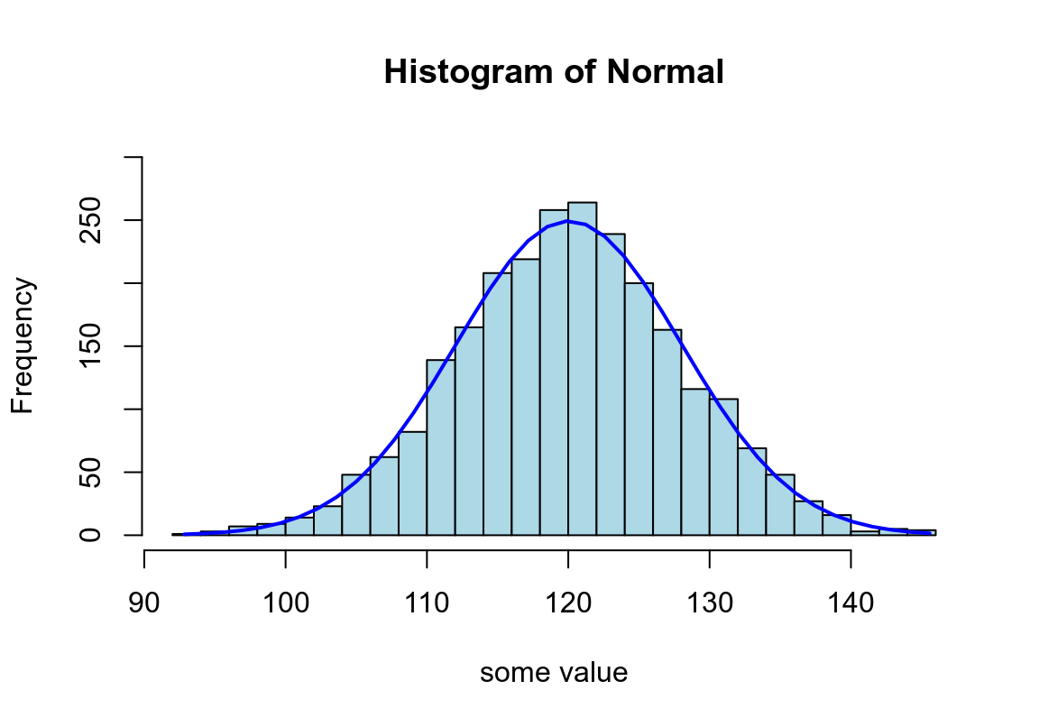
圖 25.1: Appearance of histogram with normal curve
qqnorm(Normal,frame=F); qqline(Normal)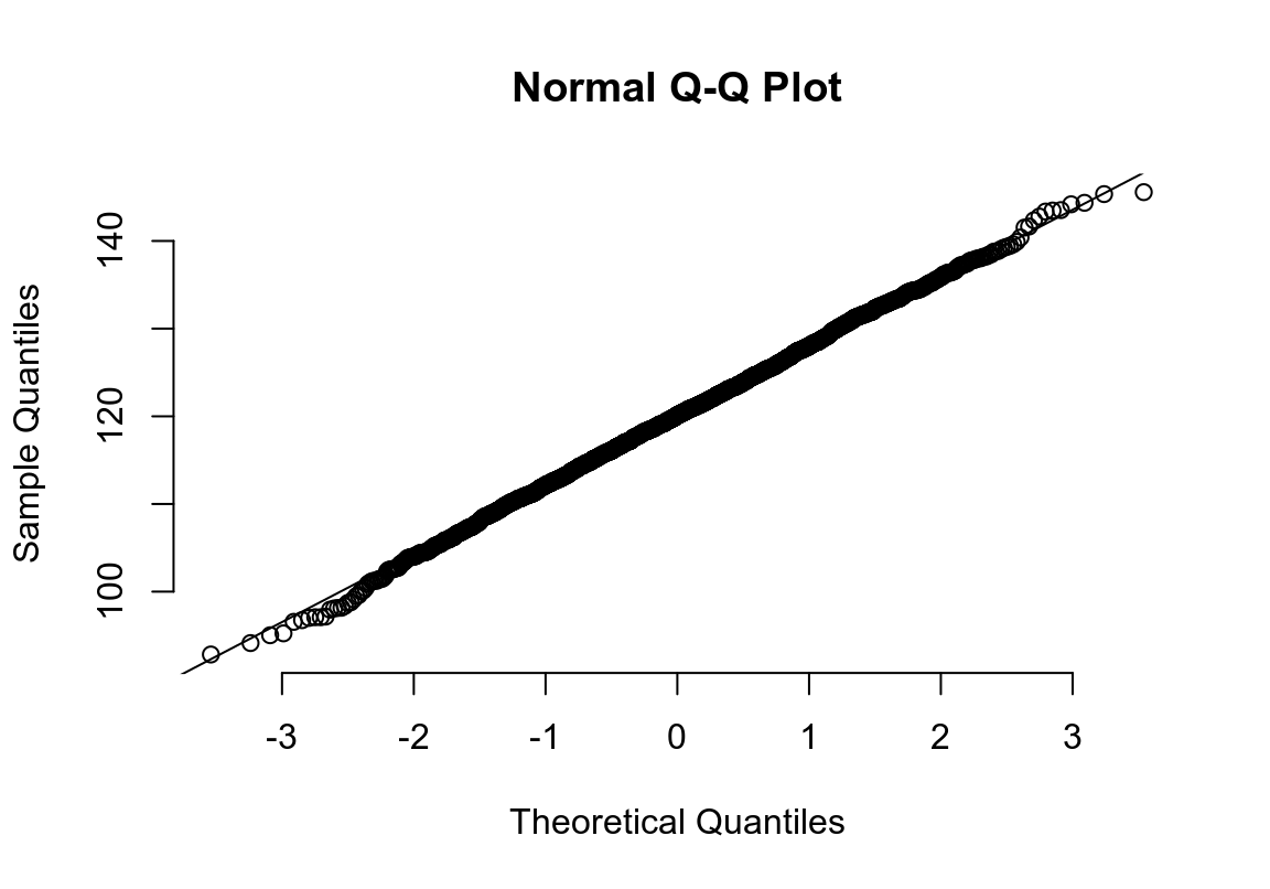
圖 25.2: Appearance of normal plot for a normally distributed variable
25.2.1 正態分佈圖 normal plot
其實光看柱狀圖和箱形圖,有時候很難判斷數據正態性與否,當數據和正態分佈有些微妙的不同時可能就沒辦法從柱狀圖覺察出來。此時需要借用正態分布圖的威力。正態分布圖的原理就是,把原始數據 (Y軸) 和理論上服從正態分佈的期待數據 (X軸) 從小到大排序一一對應以後繪製散點圖。所以理論上,如果原始數據服從正態分佈,那麼正態分佈中第10百分位的點,我們期望和原始數據中第10百分位的點十分接近,那麼繪成的散點圖應該接近於完美的貼在 \(y=x\) 這條直線上。如果正態分布圖的點越偏離 \(y=x\) 的直線,覺說明原始數據越偏離正態分佈。
下面的系列圖25.3,25.4,25.5,25.5展示了各種非正態分佈時會出現的柱狀圖,和正態分布圖的特徵:
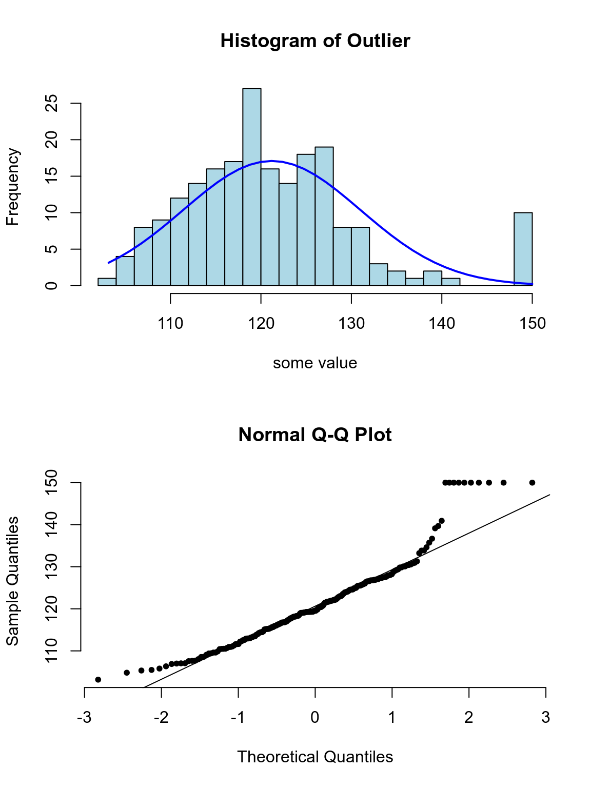
圖 25.3: Appearance of histogram and normal plot for a variable with outlying values
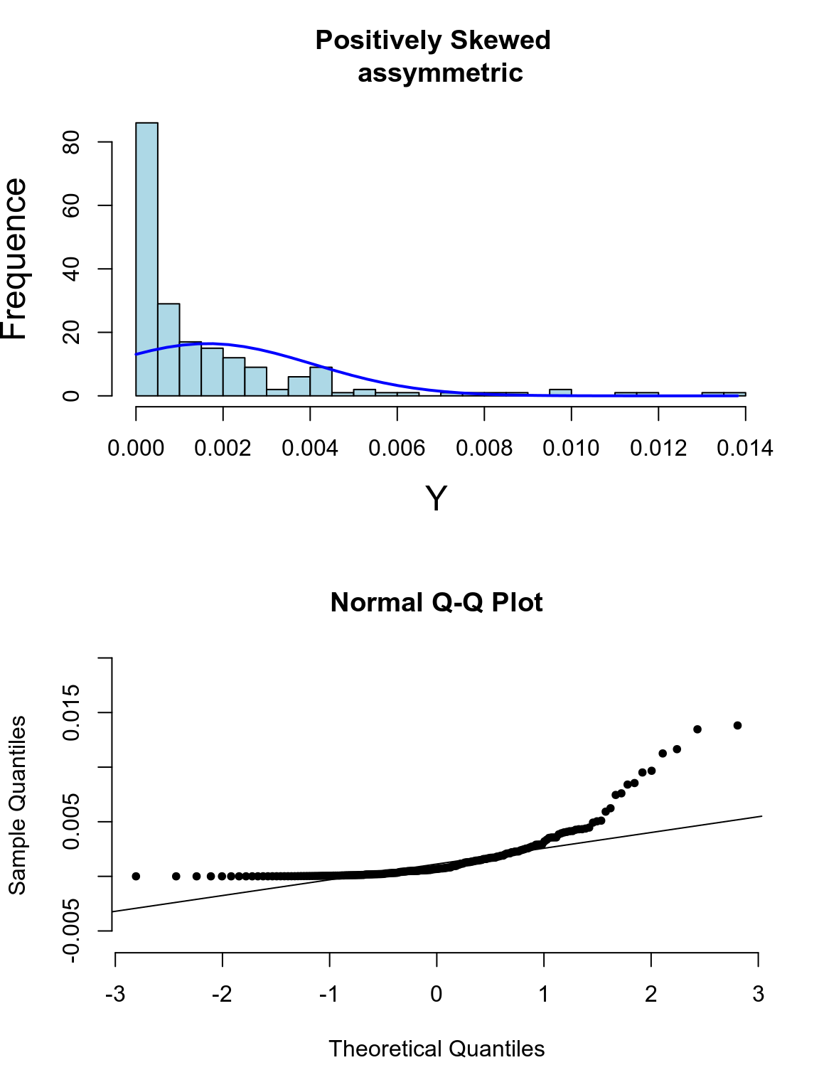
圖 25.4: Appearance of histogram and normal plot for a variable exhibiting right-skewness
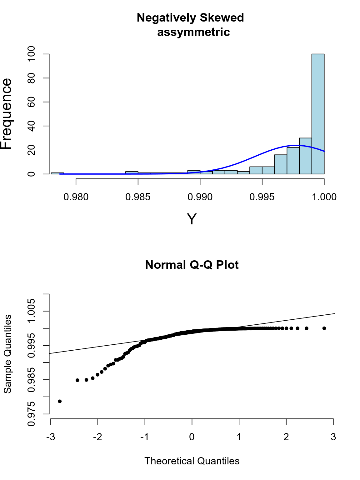
圖 25.5: Appearance of histogram and normal plot for a variable exhibiting left-skewness
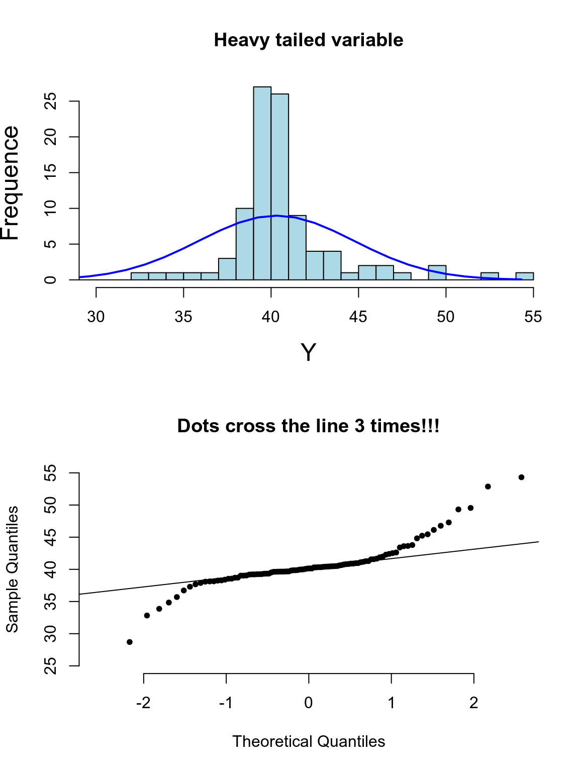
圖 25.6: Appearance of histogram and normal plot for a heavy tailed variable
如果對數據是否服從正態分佈實在沒有信心,統計學家也很少使用那些檢驗是否服從正態分佈的所謂檢驗方法 (Sharpiro-Wilk test 或者 Kolmogorov-Smirnov test),而是傾向用直接改用穩健統計學分析法 (Robust Statistical Methods)。
25.3 總結連續型變量不服從正態分佈時的處理方案
- 根據中心極限定理,樣本量足夠大時,即使原始樣本數據不服從正態分佈,仍然可以用一般的參數估計技巧來分析類似均值這樣較爲穩健的參數。
- 用非參數檢驗法,會在穩健統計學方法中介紹,但是這些方法的缺點很明顯,例如無法進行精確的參數估計,且容易失去較大的統計學檢驗力 (loss of power),增加一類錯誤概率 (錯誤的拒絕掉可能存在有意義差異的檢驗)。更重要的是,沒有一種非參數檢驗法是可以和多重線性迴歸等較爲複雜,高級的技巧等價的。
- 用一些穩健統計學方法 (bootstrap,“sandwich” estimators of variance),可行但是對電腦的計算需求較高。
- 數據轉換法。但是沒有人能保證一定能找到合適的數學轉換法來滿足前提條件 (下節討論)。
25.4 數學冪轉換 power transformations
數據轉換家族:
\[ \cdots,x^{-2},x^{-1},x^{-\frac{1}{2}},\text{log}(x),x^{\frac{1}{2}},x^1,x^2,\cdots \]
上面舉例的數學冪轉換方法,都是常見的手段用於降低原始數據的偏度 (skewness),相反地,冪轉換卻不一定能夠改變數據的峯度 (kurtosis)。下面的方程,(非常的羅嗦的方程 sorry),用於實施類似 ladder 在 Stata 中的效果,即對數據進行各種轉換,然後輸出每種冪轉換後的數據是否爲正態分佈的檢驗結果 (使用 shapiro.test()):
Ladder.x <- function(x){
    data <- data.frame(x^3,x^2,x,sqrt(x),log(x),1/sqrt(x),1/x,1/(x^2),1/(x^3))
    names(data) <- c("cubic","square","identity","square root","log","1/(square root)",
                     "inverse","1/square","1/cubic")
   # options(scipen=5)
    test1 <- shapiro.test(data$cubic)
    test2 <- shapiro.test(data$square)
    test3 <- shapiro.test(data$identity)
    test4 <- shapiro.test(data$`square root`)
    test5 <- shapiro.test(data$log)
    test6 <- shapiro.test(data$`1/(square root)`)
    test7 <- shapiro.test(data$inverse)
    test8 <- shapiro.test(data$`1/square`)
    test9 <- shapiro.test(data$`1/cubic`)
    W.statistic <- c(test1$statistic,
                     test2$statistic,
                     test3$statistic,
                     test4$statistic,
                     test5$statistic,
                     test6$statistic,
                     test7$statistic,
                     test8$statistic,
                     test9$statistic)
    p.value <- c(test1$p.value,
                 test2$p.value,
                 test3$p.value,
                 test4$p.value,
                 test5$p.value,
                 test6$p.value,
                 test7$p.value,
                 test8$p.value,
                 test9$p.value)
    Hmisc::format.pval(p.value ,digits=5, eps = 0.00001, scientific = FALSE)
    Transformation <- c("cubic","square","identity","square root","log","1/(square root)",
                        "inverse","1/square","1/cubic")
    Formula <- c("x^3","x^2","x","sqrt(x)","log(x)","1/sqrt(x)","1/x","1/(x^2)","1/(x^3)")
    (results <- data.frame(Transformation, Formula, W.statistic, p.value))
  }
Normal <- rnorm(2500, mean = 120, sd = 8)
Ladder.x(Normal)## Transformation Formula W.statistic p.value
## 1 cubic x^3 0.9901 3.906e-12
## 2 square x^2 0.9968 4.283e-05
## 3 identity x 0.9994 5.835e-01
## 4 square root sqrt(x) 0.9990 2.039e-01
## 5 log log(x) 0.9977 8.750e-04
## 6 1/(square root) 1/sqrt(x) 0.9952 3.370e-07
## 7 inverse 1/x 0.9917 8.896e-11
## 8 1/square 1/(x^2) 0.9816 1.735e-17
## 9 1/cubic 1/(x^3) 0.9674 2.175e-2325.4.1 對數轉換 logarithmic Transformation
在衆多冪轉換中,對數轉換是最常用的,因爲對數轉換之後,再通過逆運算轉換回原單位數據的方法,被發現是相較於其他冪轉換較爲容易解釋和應用在臨牀醫學中。假如現在在分析男女之間收縮期血壓的均值差別。下面是對數轉換前後的檢驗方法步驟,試作一個對比:
轉換前:
- 計算收縮期血壓在男性女性中各自的均值 \(\bar{Y}_j, j=1,2\);
- 計算男女間均值差 \(D=\bar{Y}_2 - \bar{Y}_1\);
- 所以均值差就被解釋爲男女減血壓的平均差距 (difference of mmHg);
- 例如,均值差爲 10 mmHg,就可以被解讀爲女性血壓平均值比男性低 10 mmHg。
對數轉換後:
- 計算觀察值的對數值 \(t_{ij} = \text{log}_e(y_{ij})\);
- 計算男女對數收縮期血壓的算數平均值 \(\bar{T}_j, j=1,2\);
- 計算對數血壓均值差 \(D=\bar{T}_2-\bar{T}_1\);
- 由於 \(exp(\bar{T}_j) = G_j\) 是男女收縮期血壓的幾何平均值,所以 \(exp(D)=exp(\text{log}_eG_2 - \text{log}_eG_1) = \frac{G_2}{G_1}\),就可以解釋爲男女收縮期血壓的幾何平均值之比;
- 例如,\(D=-0.05\),那麼男女收縮期血壓的幾何平均值之比爲 \(exp(-0.05)=0.951\),就可以被解讀爲女性收縮期血壓平均比男性低 \(4.9\%\)。
25.4.2 逆轉換信賴區間 back-transformation of CIs
當使用轉換後數據計算信賴區間以後,需要再把數據逆轉換回原始數據的單位才能順利被解讀。但是逆轉換回去以後的信賴區間就不再左右對稱了 (no way)。
25.4.3 對數正態分佈 log-normal distribution
一個隨機變量的對數轉換如果服從正態分佈,我們說這個數據服從對數正態分佈。
25.4.4 百分比的轉換
百分比被侷限在 \([0,1]\) 的範圍內,所以爲了打破這個取值範圍的限制,百分比常用的數學轉換有:
- 把百分比 \(\pi\) 轉換成 Odds \(\frac{\pi}{1-\pi}\)。如此 Odds 的取值範圍就可以變成 \([0, \infty)\);
- Odds \(\frac{\pi}{1-\pi}\) 又常被轉換成 log-odds \(\text{log}(\frac{\pi}{1-\pi})\)。這樣的轉換方程 \(f(\pi)=\text{log}(\frac{\pi}{1-\pi})\) 又被命名爲邏輯轉換 (logit transformation);
- 百分比的商 (危險度比,risk ratio) \(\pi_1/\pi_2\) 可以轉換成 \(\text{log}(\pi_1/\pi_2)\);
- 比值比 (odds ratio) \(\frac{\pi_1(1-\pi_2)}{\pi_2(1-\pi_1)}\) 可以轉換成對數比值比 (log odds ratio) \(\text{log}[\frac{\pi_1(1-\pi_2)}{\pi_2(1-\pi_1)}] = \text{log}[\pi_1(1-\pi_1)] - \text{log}[\pi_2(1-\pi_2)]\)。
| Transformation | Formula | Range |
|---|---|---|
| Odds | \(\frac{\pi}{1-\pi}\) | \([0,\infty)\) |
| Log Odds | \(\text{log}(\frac{\pi}{1-\pi})\) | \((-\infty,+\infty)\) |
| Risk Ratio | \(\frac{\pi_1}{\pi_2}\) | \([0,\infty)\) |
| Log Risk Ratio | \(\text{log}(\frac{\pi_1}{\pi_2})\) | \((-\infty,+\infty)\) |
| Odds Ratio | \(\frac{\pi_1(1-\pi_2)}{\pi_2(1-\pi_1)}\) | \([0,\infty)\) |
| Log Odds Ratio | \(\text{log}[\frac{\pi_1(1-\pi_2)}{\pi_2(1-\pi_1)}]\) | \((-\infty,+\infty)\) |
References
Belle, G. van, L.D. Fisher, P.J. Heagerty, and T. Lumley. 2004. Biostatistics: A Methodology for the Health Sciences. Wiley Series in Probability and Statistics. Wiley. https://books.google.co.uk/books?id=KSh8IOrLPzwC.