第 59 章 隨機截距模型 random intercept model
最簡單的隨機效應模型 – 隨機截距模型 random intercept model。
59.1 隨機截距模型的定義
有時,我們對每個分層各自的截距大小並不那麼感興趣,且如果只有固定效應的話,其實我們從某種程度上忽略掉了數據層與層之間變異的方差 (between cluster variation)。於是,在模型中考慮這些問題的解決方案就是 – 我們讓各層的截距呈現隨機效應 (treat the variation in cluster intercepts not as fixed),把這些截距視爲來自與某種分布的隨機呈現 (randomly draws from some distribution)。於是原先的只有固定效應部分的模型,就增加了隨機截距部分:
\[ \begin{aligned} Y_{ij} & = \mu + u_j + \varepsilon_{ij} \\ \text{where } u_j & \stackrel{N.I.D}{\sim} N(0, \sigma_u^2) \\ \varepsilon_{ij} & \stackrel{N.I.D}{\sim} N(0, \sigma_\varepsilon^2) \\ u_j & \text{ are independent from } \varepsilon_{ij} \\ \end{aligned} \tag{59.1} \]
這個混合效應模型中,
- \(\mu\) 是總體均值;
- \(u_j\) 是一個服從均值 0, 方差 (the population between cluster variance) 爲 \(\sigma_u^2\) 的正態分布的隨機變量;
- \(\varepsilon_{ij}\) 是隨機誤差,它也被認爲服從均值爲 0, 方差爲 \(\sigma_\varepsilon^2\) 的正太分布,且這兩個隨機效應部分之間也是相互獨立的。
- 從該模型估算的結果變量 \(Y_{ij}\) 的方差是 \(\sigma_u^2 + \sigma_\varepsilon^2\)。
- 隨機截距模型又被叫做是 方差成分模型 (variance-component model),或者是單向隨機效應方差模型 (one-way random effects ANOVA model)。
這個模型和僅有固定效應的模型,有顯著的不同:
\[ Y_{ij} = \mu + \gamma_j + \varepsilon_{ij} \]
固定效應模型裏,
- \(\mu\) 也是總體均值;
- \(\sum_{j=1}^J \gamma_j = 0\) 是將各組不同截距之和強制爲零的過程;
所以隨機截距模型打破了這個限制,使得隨機的截距 \(\mu_j\) 成爲一個服從均值爲 0,方差爲 \(\sigma_u^2\) 的 隨機變量。
隨機效應部分 \(u_j\) 和隨機誤差 \(\varepsilon_{ij}\) 之間相互獨立的前提,意味着兩個裏屬於不同層級的觀察之間是相互獨立的,但是反過來,同屬於一個層級的個體之間就變成了有相關性的了 (within cluster correlation):
\[ \begin{aligned} \because Y_{1j} & = \mu + u_j + \varepsilon_{1j} \\ Y_{2j} & = \mu + u_j + \varepsilon_{2j} \\ \therefore \text{Cov}(Y_{1j}, Y_{2j}) & = \text{Cov}(u_j, u_j) + \text{Cov}(u_j, \varepsilon_{2j}) + \text{Cov}(\varepsilon_{1j}, u_j) + \text{Cov}(\varepsilon_{1j}, \varepsilon_{2j}) \\ & = \text{Cov}(u_j, u_j) = V(u_j, u_j)\\ & = \sigma_u^2 \end{aligned} \]
由於 \(\text{Var}(Y_{1j}) = \text{Var}(Y_{2j}) = \sigma_u^2 + \sigma_\varepsilon^2\),所以,同屬一層的兩個個體之間的層內相關系數 (intra-class correlation):
\[ \lambda = \frac{\text{Cov}(Y_{1j}, Y_{2j})}{\text{SD}(Y_{1j})\text{SD}(Y_{2j})} = \frac{\sigma_u^2}{\sigma_\varepsilon^2 + \sigma_u^2} \]
從層內相關系數的公式也可看出,該相關系數可以同時被理解爲結果變量 \(Y_{ij}\) 的方差中歸咎與層(cluster)結構的部分的百分比。
This is the within-cluster or intra-class correlation, that we will denote \(\lambda\). Note that it is also the proportion of total variance that is accounted for by the cluster.
59.2 隨機截距模型的參數估計
如此,我們就知道在隨機截距模型裏,有三個需要被估計的參數 \(\mu, \sigma_u^2, \sigma^2_\varepsilon\)。我們可以利用熟悉的極大似然估計法估計這些參數 (Maximum Likelihood, ML)。當且進當嵌套式結構數據是平衡數據 (balanced)時 (即,每層中的個體數量相同),這三個參數的 \(\text{MLE}\) 分別是:
\[ \begin{aligned} \hat\mu & = \bar{Y} \\ \hat\sigma_\varepsilon^2 & = \text{Mean square error, MSE} \\ \hat\sigma_u^2 & = \frac{\text{Model Sum of Squares, MSS}}{Jn} - \frac{\hat\sigma^2_\varepsilon}{n} \end{aligned} \tag{59.2} \]
只要模型指定正確無誤,前兩個極大似然估計是他們各自的無偏估計。但第三個,也就是層內方差的估計量確實際上是低估了的 (downward biased)。這裏常用的另一種對層內方差參數的估計法被叫做矩估計量 (moment estimator, or ANOVA estimator):
\[ \begin{aligned} \widetilde{\sigma}_u^2 & = \frac{\text{MSS}}{(J-1)n}- \frac{\hat\sigma_\varepsilon^2}{n} \\ & = \frac{\text{MSS} - \text{MSE}(J-1)}{(J-1)n} \\ & = \frac{\text{MMS}(J-1) - \text{MSE}(J-1)}{(J-1)n} \\ & = \frac{\text{MMS} - \text{MSE}}{n} \end{aligned} \]
對於平衡數據 (balanced data),這個矩估計量又被叫做限制性極大似然 (Restricted Maximum Likelihood, REML)。限制性極大似然法,是一個真極大似然過程 (genuine maximum likelihood procedure),但是它每次進行估計的時候,會先“去除掉”固定效應部分,所以每次用於估計參數的數據其實是對數據的線性轉換後 \(Y_{ij} - \mu = u_j + \varepsilon_{ij}\),它使用的數據是這個等式右半部分的轉換後數據。在 REML 過程中,先估計層內方差 \(\sigma_u^2\) 再對固定效應部分的總體均值估計,所以是個兩步走的過程。另外除了這裏討論的 ML, REML這兩種對層內方差進行參數估計的方法之外,在計量經濟學 (econometrics) 中常用的是 (本課不深入探討) 廣義最小二乘法 (Generalized Least Squares, GLS)。GLS 使用的是一種加權的最小二乘法 (OLS),該加權法根據層與隨機誤差的方差成分 (variance components) 不同而給不同的層以不同的截距權重。當數據本身是平衡數據時,GLS給出的估計結果等同於 REML法。當數據不是平衡數據的時候,ML/REML 其實背後使用的原理也是 GLS。
59.3 如何在 R 中進行隨機截距模型的擬合
在 R 或 STATA 中擬合隨機截距模型,需要數據爲“長 (long)” 數據,下面的代碼可以在 R 裏面把 “寬 (wide)” 的數據調整成爲 長 數據:
pefr <- read_dta("backupfiles/pefr.dta")
# the data are in wide format
head(pefr)
## # A tibble: 6 x 5
## id wp1 wp2 wm1 wm2
## <dbl> <dbl> <dbl> <dbl> <dbl>
## 1 1 494 490 512 525
## 2 2 395 397 430 415
## 3 3 516 512 520 508
## 4 4 434 401 428 444
## 5 5 476 470 500 500
## 6 6 557 611 600 625# transform data into long format
pefr_long <- pefr %>%
gather(key, value, -id) %>%
separate(key, into = c("measurement", "occasion"), sep = 2) %>%
arrange(id, occasion) %>%
spread(measurement, value)
pefr_long## # A tibble: 34 x 4
## id occasion wm wp
## <dbl> <chr> <dbl> <dbl>
## 1 1 1 512 494
## 2 1 2 525 490
## 3 2 1 430 395
## 4 2 2 415 397
## 5 3 1 520 516
## 6 3 2 508 512
## 7 4 1 428 434
## 8 4 2 444 401
## 9 5 1 500 476
## 10 5 2 500 470
## # ... with 24 more rows在 R 裏面,有兩個包 (lme4::lmer 或 nlme::lme) 的各自兩種代碼以供選用:
M0 <- lme(fixed = wm ~ 1, random  = ~ 1 | id, data = pefr_long, method = "REML")
summary(M0)
## Linear mixed-effects model fit by REML
## Data: pefr_long
## AIC BIC logLik
## 366.75843 371.24795 -180.37921
##
## Random effects:
## Formula: ~1 | id
## (Intercept) Residual
## StdDev: 110.39701 19.910835
##
## Fixed effects: wm ~ 1
## Value Std.Error DF t-value p-value
## (Intercept) 453.91176 26.992068 17 16.816487 0
##
## Standardized Within-Group Residuals:
## Min Q1 Med Q3 Max
## -2.444435579 -0.335076940 0.037044891 0.350983659 2.377059741
##
## Number of Observations: 34
## Number of Groups: 17M1 <- lmer(wm ~ (1|id), data = pefr_long, REML = TRUE)
summary(M1)## Linear mixed model fit by REML. t-tests use Satterthwaite's method ['lmerModLmerTest']
## Formula: wm ~ (1 | id)
## Data: pefr_long
##
## REML criterion at convergence: 360.8
##
## Scaled residuals:
## Min 1Q Median 3Q Max
## -2.444436 -0.335077 0.037045 0.350984 2.377060
##
## Random effects:
## Groups Name Variance Std.Dev.
## id (Intercept) 12187.51 110.397
## Residual 396.44 19.911
## Number of obs: 34, groups: id, 17
##
## Fixed effects:
## Estimate Std. Error df t value Pr(>|t|)
## (Intercept) 453.912 26.992 16.000 16.817 1.36e-11 ***
## ---
## Signif. codes: 0 '***' 0.001 '**' 0.01 '*' 0.05 '.' 0.1 ' ' 1不知道爲什麼在 R 裏有這兩種完全不同的方式來擬合混合效應模型。還好他們的結果基本完全一致。在這個極爲簡單的例子裏,我們可以利用模型擬合的結果中 Random effects 的部分來計算層內相關系數 (intra-class correlation):
\[ \hat\lambda = \frac{\hat\sigma_u^2}{(\hat\sigma_u^2 + \hat\sigma_\varepsilon^2)} = \frac{110.40^2}{110.40^2 + 19.91^2} = 0.97 \]
這是對 Mini Wright meter 測量方法可靠性的一個評價指標。其中 \(\sigma_u^2\) 是患者最大呼吸速率 (PEFR) 測量值的方差,\(\sigma_\varepsilon^2\) 是測量的隨機誤差,所以這裏的測量方法的可靠度是 97%,是可信度十分高的測量準確度。
59.4 隨機截距模型中的統計推斷
59.4.1 固定效應部分的推斷
當數據是平衡數據時,固定效應的 \(\mu\) 的 \(\text{MLE}\) 是總體的均值 (overall mean)。它的估計標準誤是:
\[ \hat{\text{SE}}(\hat\mu) = \sqrt{\frac{n\hat\sigma_u^2 + \hat\sigma_\varepsilon^2}{Jn}} \]
記得線性回歸中(固定效應模型中),\(\mu\) 的 \(\text{MLE}\) 也還是總體的均值 (overall mean)。它的估計標準誤卻是:
\[ \hat{\text{SE}}(\hat\mu^F) = \sqrt{\frac{\hat\sigma_\varepsilon^2}{Jn}} \]
所以,僅有固定效應模型時的總體均值的標準誤總是要比混合效應模型下估計的總體均值標準誤要小
\[ \hat{\text{SE}}(\hat\mu^F) < \hat{\text{SE}}(\hat\mu) \]
如果數據不是平衡數據,那麼隨機截距模型中 \(\mu\) 的 \(\text{MLE}\) 是每層均值的加權均值 (a weighted mean of the cluster specific means):
\[ \begin{aligned} \hat\mu & = \frac{\sum_jw_j\bar{Y}_{\cdot j}}{\sum_j w_j} \\ \text{Where } w_j & = \frac{1}{\sigma_u^2 + \sigma_\varepsilon^2/n_j} \end{aligned} \]
從加權的方式來看,如果樣本量少的層級數據本身的誤差方差 \(\sigma_\varepsilon^2\) 也較小,那麼層樣本量較小的層也會和層樣本量較大的層獲得相似的均值權重。
零假設是 \(\mu = 0\) 的檢驗,就計算 \(z\) 檢驗統計量就可以 (或者 \(z^2\) 的 Wald 檢驗):
\[ z = \frac{\hat\mu}{\hat{\text{SE}}(\hat\mu)} \] 總體均值的 95% 信賴區間的計算式就是:
\[ \hat\mu \pm z_{0.975}\hat{\text{SE}}(\hat\mu) \]
59.4.2 隨機效應部分的推斷
總體均值的假設檢驗搞定了之後,我們肯定還想對隨機截距模型擬合的隨機效應方差作出是否有意義的假設檢驗。也就是我們希望能檢驗零假設 \(\sigma_u^2 = 0\),和替代假設 \(\sigma_u^2 > 0\)。一般情況下大家肯定會想到對含有隨機效應的模型和只有固定效應的模型使用 LRT (似然比檢驗),然後把檢驗統計量拿去和自由度爲 1 的卡方分布做比較。但是其實方差本身永遠都是大於等於零的,所以傳統的 LRT 在這個零假設時並不適用。
在零假設條件下 \(\sigma_u^2 = 0\),也就是說層內相關在一半的數據中是正相關,另一半數據中是正好相反的負相關,以此相互抵消,方差爲零。所以其實這裏的 LRT 檢驗統計量應該服從的不是自由度爲 1 的卡方分布那麼簡單,而是一種混合卡方分布 (自由度 1 和 自由度爲 0 的混合卡方分布 \(\chi_{0,1}^2\))。所以應該把模型比較之後計算獲得的 \(p\) 值除以2,以獲得準確的對 \(\sigma_u^2 = 0\) 檢驗的 \(p\) 值。
M0 <- lme(fixed = wm ~ 1, random  = ~ 1 | id, data = pefr_long, method = "REML")
M0_fixed<- lm(wm ~ 1, data = pefr_long)
anova(M0, M0_fixed)
## Model df AIC BIC logLik Test L.Ratio p-value
## M0 1 3 366.75843 371.24795 -180.37921
## M0_fixed 2 2 411.71916 414.71217 -203.85958 1 vs 2 46.960731 <.0001回到本例中的混合效應模型和固定效應模型的比較來看,LRT本身的 P 值已經 \(<0.0001\),所以除不除以二對推斷結果都沒有太大影響。也就是本例中的隨即截距模型是比固定效應的簡單線性回歸模型更加適合該數據的模型。
其他注意點:
- 在坑爹的 STATA 裏面混合效應模型居然還會輸出隨機效應方差的 “標準誤”,該數字請你無視之。
- 當樣本擁有足夠多的樣本量 (其實是第二階層的層數),極大似然法 (ML) 和限制性極大似然法 (REML) 給出的結果會相當接近。
- 當你比較兩個不是互爲嵌套 (nested) 的模型時,可以使用 AIC/BIC 指標。
59.5 練習題
59.5.1 數據
- GHQ 數據
該數據包含 12 名學生前後兩次回答 General Health Questionnaire (GHQ) 問卷獲得的數據。該問卷用於測量學生的心理壓力,其變量名和含義如下:
id        Student identifier
GHQ1      General Health Questionnaire score- 1st occasion
GHQ2 General Health Questionnaire score- 2nd occasion- Siblings 數據
該數據是來自一項對 3978 名媽媽關於她們 8604 名孩子的出生體重及健康狀況的問卷調查。該數據的變量名和含義如下:
momid     Mother identifier
idx       Baby identifier
mage      Maternal age (years)
meduc     Maternal education
gestat    gestational age (weeks)
birwt     Birth weight (g)
smoke     Maternal smoking (0 = no, 1 = yes)
male      Baby boy (0 = no, 1 = yes)
year      Year of birth
married   Maternal marital status (0 = no, 1 = yes)
hsgrad    Maternal high school education (0 = no, 1 = yes)
black     Maternal race (1 = black, 0 = other)
59.5.2 讀入 GHQ 數據,探索其內容,該數據是否是平衡數據 (balanced)?計算每名學生的兩次問卷成績平均分。
ghq <- read_dta("backupfiles/ghq.dta")
ghq
## # A tibble: 12 x 3
## id GHQ1 GHQ2
## <dbl> <dbl> <dbl>
## 1 1 12 12
## 2 2 8 7
## 3 3 22 24
## 4 4 10 14
## 5 5 10 8
## 6 6 6 4
## 7 7 8 5
## 8 8 4 6
## 9 9 14 14
## 10 10 6 5
## 11 11 2 5
## 12 12 22 16ghq <- ghq %>%
mutate(mean = (GHQ1 + GHQ2)/2)
# each student has 2 observations (i.e. n_j = n = 2)
# and therefore the data are balanced.
# the overall mean is 10.167 and its SD is 6.073
with(ghq, summ(mean, graph = FALSE))## obs. mean median s.d. min. max.
## 12 10.167 8.25 6.073 3.5 2359.5.3 把數據從寬 (wide) 改變成長 (long) 的形式
# transform data into long format
ghq_long <- ghq %>%
  gather(key, value, -id, -mean) %>%
  separate(key, into = c("measurement", "occasion"), sep = 3) %>%
  arrange(id, occasion) %>%
  spread(measurement, value)
ghq_long
## # A tibble: 24 x 4
## id mean occasion GHQ
## <dbl> <dbl> <chr> <dbl>
## 1 1 12 1 12
## 2 1 12 2 12
## 3 2 7.5 1 8
## 4 2 7.5 2 7
## 5 3 23 1 22
## 6 3 23 2 24
## 7 4 12 1 10
## 8 4 12 2 14
## 9 5 9 1 10
## 10 5 9 2 8
## # ... with 14 more rows# after reshaping there are 24 records. the summary statistics are
# overall mean sd and min max
with(ghq_long, summ(GHQ, graph = FALSE))## obs. mean median s.d. min. max.
## 24 10.167 8 6.098 2 24# between groups mean sd and min
summ(ghq_long[!duplicated(ghq_long$id), ]$mean, graph = FALSE)## obs. mean median s.d. min. max.
## 12 10.167 8.25 6.073 3.5 23# within groups mean sd and min (came from the difference between
# the overall mean and the within difference) observations for
# each group = 2
ghq_long <- ghq_long %>%
mutate(dif_GHQ = mean(GHQ) - (GHQ - mean))
with(ghq_long, summ(dif_GHQ, graph = FALSE))## obs. mean median s.d. min. max.
## 24 10.167 10.167 1.383 7.167 13.167GHQ 的分佈並不左右對稱。
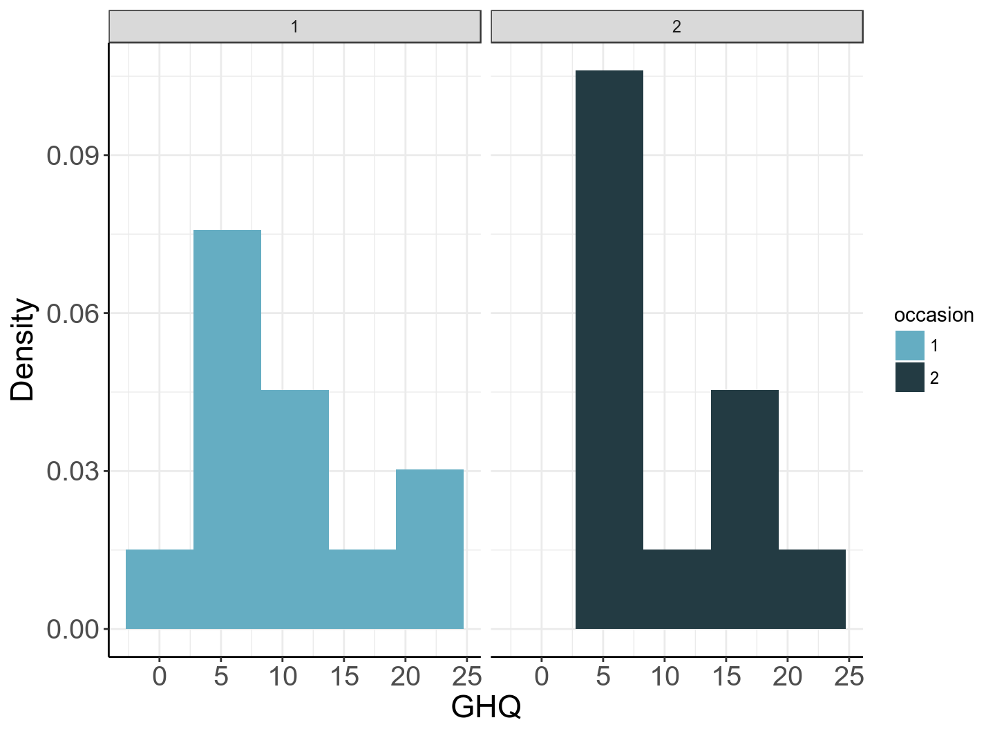
圖 59.1: Histogram of GHQ by occasion
59.5.4 對數據按照 id 分層進行 ANOVA
with(ghq_long, anova(lm(GHQ~factor(id))))## Analysis of Variance Table
##
## Response: GHQ
## Df Sum Sq Mean Sq F value Pr(>F)
## factor(id) 11 811.333 73.7576 20.1157 4.7782e-06 ***
## Residuals 12 44.000 3.6667
## ---
## Signif. codes: 0 '***' 0.001 '**' 0.01 '*' 0.05 '.' 0.1 ' ' 1#library(lme4)
( fit <- lmer(GHQ ~ (1|id), data=ghq_long) )## Linear mixed model fit by REML ['lmerModLmerTest']
## Formula: GHQ ~ (1 | id)
## Data: ghq_long
## REML criterion at convergence: 131.3492
## Random effects:
## Groups Name Std.Dev.
## id (Intercept) 5.9199
## Residual 1.9149
## Number of obs: 24, groups: id, 12
## Fixed Effects:
## (Intercept)
## 10.167\(\sigma_u, \sigma_e\) 的估計值分別是 5.92 (between), 1.91 (within)。可以計算層間相關係數 (intra-class correlation) \(\hat\lambda = \frac{\sigma^2_u}{\sigma^2_u + \sigma^2_e} = 0.905\)。且 \(\hat\sigma_u = \sqrt{\frac{73.8 - 3.7}{2}} = 5.92\),和前一次練習一樣地,這個隨機效應的方差,可以通過方差分析表格來直接手動計算 (當且僅當分層數據是平衡狀態的)。和前面計算的樣本數據比較,樣本層間標準差是高估了的 (sample between variance = 6.073 > 5.92),相反樣本層內標準差 (within sd) 則是低估了的 (sample within sd = 1.383 < 1.91)。兩個層內標準差的關係是:
\[ \sqrt{1.383^2\times\frac{23}{12}} = 1.91 \]
59.5.5 用 R 裏的 nlme 包,使用限制性極大似然法 (restricted maximum likelihood, REML) 擬合截距混合效應模型,比較其結果和前文中隨機效應 ANOVA 的結果
summary(nlme::lme(fixed = GHQ ~ 1, random = ~ 1 | id, data = ghq_long, method = "REML"))## Linear mixed-effects model fit by REML
## Data: ghq_long
## AIC BIC logLik
## 137.34924 140.75573 -65.674622
##
## Random effects:
## Formula: ~1 | id
## (Intercept) Residual
## StdDev: 5.9199181 1.9148548
##
## Fixed effects: GHQ ~ 1
## Value Std.Error DF t-value p-value
## (Intercept) 10.166667 1.7530632 12 5.7993727 0.0001
##
## Standardized Within-Group Residuals:
## Min Q1 Med Q3 Max
## -1.337372043 -0.578482697 0.073557531 0.414059981 1.796024881
##
## Number of Observations: 24
## Number of Groups: 12截距混合效應模型的參數估計和隨機效應 ANOVA 的參數估計是一樣的。
59.5.6 用極大似然法 (maximum likelihood, ML) method = "ML" 重新擬合前面的混合效應模型,比較結果有什麼不同。
#( fit <- lmer(GHQ ~ (1|id), data=ghq_long, REML = FALSE) ) # same but from `lme4` package

summary(lme(fixed = GHQ ~ 1, random = ~ 1 | id, data = ghq_long, method = "ML"))
## Linear mixed-effects model fit by maximum likelihood
## Data: ghq_long
## AIC BIC logLik
## 140.26571 143.79987 -67.132857
##
## Random effects:
## Formula: ~1 | id
## (Intercept) Residual
## StdDev: 5.6543976 1.9148545
##
## Fixed effects: GHQ ~ 1
## Value Std.Error DF t-value p-value
## (Intercept) 10.166667 1.7145299 12 5.929711 0.0001
##
## Standardized Within-Group Residuals:
## Min Q1 Med Q3 Max
## -1.31652454 -0.58359637 0.08024454 0.40422622 1.81687284
##
## Number of Observations: 24
## Number of Groups: 12用極大似然法估計的隨機殘差標準差 \(\sigma_e\) 和 REML/ANOVA 法估計的相同,但是隨機效應標準差 \(\sigma_u\) 略小 5.65 < 5.92。
59.5.7 用簡單線性迴歸擬合一個固定效應模型
Fixed_reg <- lm(GHQ-mean(GHQ) ~ 0 + factor(id), data = ghq_long)
summary(Fixed_reg)
##
## Call:
## lm(formula = GHQ - mean(GHQ) ~ 0 + factor(id), data = ghq_long)
##
## Residuals:
## Min 1Q Median 3Q Max
## -3 -1 0 1 3
##
## Coefficients:
## Estimate Std. Error t value Pr(>|t|)
## factor(id)1 1.8333 1.3540 1.3540 0.2006847
## factor(id)2 -2.6667 1.3540 -1.9695 0.0724256 .
## factor(id)3 12.8333 1.3540 9.4780 6.371e-07 ***
## factor(id)4 1.8333 1.3540 1.3540 0.2006847
## factor(id)5 -1.1667 1.3540 -0.8616 0.4057744
## factor(id)6 -5.1667 1.3540 -3.8158 0.0024580 **
## factor(id)7 -3.6667 1.3540 -2.7080 0.0190252 *
## factor(id)8 -5.1667 1.3540 -3.8158 0.0024580 **
## factor(id)9 3.8333 1.3540 2.8311 0.0151447 *
## factor(id)10 -4.6667 1.3540 -3.4466 0.0048356 **
## factor(id)11 -6.6667 1.3540 -4.9237 0.0003516 ***
## factor(id)12 8.8333 1.3540 6.5238 2.836e-05 ***
## ---
## Signif. codes: 0 '***' 0.001 '**' 0.01 '*' 0.05 '.' 0.1 ' ' 1
##
## Residual standard error: 1.9149 on 12 degrees of freedom
## Multiple R-squared: 0.94856, Adjusted R-squared: 0.89712
## F-statistic: 18.439 on 12 and 12 DF, p-value: 6.8362e-06可以看到輸出報告最底段部分 Residual standard error: 1.91 on 12 degrees of freedom 就是前文三種不同模型擬合的隨機殘差效應的標準差。在 STATA 裏被叫做 Root MSE。
59.5.8 計算這些隨機截距的均值和標準差
summ(Fixed_reg$coefficients, graph = FALSE)## obs. mean median s.d. min. max.
## 12 0 -1.917 6.073 -6.667 12.833這裏僅僅用固定效應模型時,不同羣截距的均值雖然和用混合效應模型估計的一樣爲零,但是其估計的標準差要大於無論是 REML (5.92) 或者是 ML (5.65) 估計值的大小,其實這裏簡單線性迴歸給出的截距均值,就是本練習一開始讓你計算的樣本均值的標準差 (between group sd)。這是因爲簡單線性迴歸 (固定效應模型) 忽視了這些不同組的均值的不確定性。
59.5.9 忽略掉所有的分層和解釋變量擬合 GHQ 的簡單線性迴歸
Fixed_simple <- lm(GHQ ~ 1, data = ghq_long)
summary(Fixed_simple)
##
## Call:
## lm(formula = GHQ ~ 1, data = ghq_long)
##
## Residuals:
## Min 1Q Median 3Q Max
## -8.1667 -4.4167 -2.1667 3.8333 13.8333
##
## Coefficients:
## Estimate Std. Error t value Pr(>|t|)
## (Intercept) 10.1667 1.2448 8.1673 3.001e-08 ***
## ---
## Signif. codes: 0 '***' 0.001 '**' 0.01 '*' 0.05 '.' 0.1 ' ' 1
##
## Residual standard error: 6.0982 on 23 degrees of freedom此時的模型估計的 Residual standard error: 6.09 on 23 degrees of freedom 其實就是一開始讓你計算的樣本整體的標準差 (overall sd)
59.5.10 用分層的穩健法 (三明治標準誤法) 計算簡單線性迴歸時,截距的標準誤差,和簡單線性迴歸時的結果作比較
# sandwich robust method with cluster id

robustReg <- clubSandwich::coef_test(Fixed_simple, vcov = "CR1", cluster = ghq_long$id)

rob.std.err <- robustReg$SE
naive.std.err<-summary(Fixed_simple)$coefficients[,2]
better.table <- cbind("Estimate" = coef(Fixed_simple),
                      "Naive SE" = naive.std.err,
                      "Pr(>|z|)" = 2 * pt(abs(coef(Fixed_simple)/naive.std.err), df=nrow(ghq_long)-2, lower.tail = FALSE),
                      "LL" = coef(Fixed_simple) - 1.96 * naive.std.err,
                      "UL" = coef(Fixed_simple) + 1.96 * naive.std.err,
                      "Robust SE" = rob.std.err,
                      "Pr(>|z|)" = 2 * pt(abs(coef(Fixed_simple)/rob.std.err), df=nrow(ghq_long)-2,
lower.tail = FALSE),
                      "LL" = coef(Fixed_simple) - qt(df=robustReg$df, 0.975) * rob.std.err,
                      "UL" = coef(Fixed_simple) + qt(df=robustReg$df, 0.975) * rob.std.err)
rownames(better.table)<-c("Constant")
better.table
## Estimate Naive SE Pr(>|z|) LL UL Robust SE Pr(>|z|) LL
## Constant 10.166667 1.2447959 4.1792464e-08 7.7268666 12.606467 1.7530637 7.7968698e-06 6.3081995
## UL
## Constant 14.02513459.5.11 讀入 siblings 數據。先總結嬰兒的出生體重,思考這個數據中嬰兒出生體重之間是否可能存在關聯性?它的來源是哪裏。用這個數據擬合兩個混合效應模型 (ML, REML),不加入任何解釋變量。
siblings <- read_dta("backupfiles/siblings.dta")
Fixed_ml <- lme(fixed = birwt ~ 1, random = ~ 1 | momid, data = siblings, method = "ML")
summary(Fixed_ml)
## Linear mixed-effects model fit by maximum likelihood
## Data: siblings
## AIC BIC logLik
## 130956.97 130978.15 -65475.486
##
## Random effects:
## Formula: ~1 | momid
## (Intercept) Residual
## StdDev: 368.28656 377.65778
##
## Fixed effects: birwt ~ 1
## Value Std.Error DF t-value p-value
## (Intercept) 3467.969 7.1380683 4626 485.84138 0
##
## Standardized Within-Group Residuals:
## Min Q1 Med Q3 Max
## -6.2745852602 -0.4860398560 0.0036050084 0.5054348663 4.0506129253
##
## Number of Observations: 8604
## Number of Groups: 3978Fixed_reml <- lme(fixed = birwt ~ 1, random = ~ 1 | momid, data = siblings, method = "REML")
summary(Fixed_reml)## Linear mixed-effects model fit by REML
## Data: siblings
## AIC BIC logLik
## 130951.2 130972.38 -65472.601
##
## Random effects:
## Formula: ~1 | momid
## (Intercept) Residual
## StdDev: 368.35596 377.65768
##
## Fixed effects: birwt ~ 1
## Value Std.Error DF t-value p-value
## (Intercept) 3467.9688 7.1385551 4626 485.80822 0
##
## Standardized Within-Group Residuals:
## Min Q1 Med Q3 Max
## -6.2743063820 -0.4860194138 0.0035299824 0.5053550416 4.0503923643
##
## Number of Observations: 8604
## Number of Groups: 3978由於該數據樣本量足夠大 (混合效應模型中等同於說數據的層數足夠多),你可以看到其實 ML 法和 REML 法估計的參數結果十分地接近。