第 37 章排列置換法 Permutation procedures

37.1 背景介紹

Good(Good 2006) 曾經提出假設檢驗構建的步驟，這裡引用如下：

分析問題，確認零假設 (null hypothesis)，和可能的替代假設 (alternative hypothesis)。確認這兩種假設決定以後可能伴隨的錯誤 (The potential risk associated with a decision)；
選擇一個檢驗統計量；
計算數據給出的檢驗統計量；
確定檢驗統計量，在零假設時的樣本分佈；
用確定好的樣本分佈，以及數據給出的統計量大小，做出決策！

本章要介紹的排列置換法 (permutation)，和下一章會介紹的自助重抽法 (bootstrap) ，需要大量的計算機的計算，和較強的電腦性能。這兩種方法有一個共同的特徵，它們都利用手頭獲得的樣本數據輔助生成樣本分佈，同時對該數據的分佈或者特質不進行假設。也就是用在上面羅列步驟的第4步。其餘的步驟則與一般的參數假設檢驗完全相同。

37.2 直接上實例

之前用過的甲亢數據：

表 37.1: Serum thyroxine levels
n=16 hypothyroid children
thyr	group
34	Slight or no symptoms
45	Slight or no symptoms
49	Slight or no symptoms
55	Slight or no symptoms
58	Slight or no symptoms
59	Slight or no symptoms
60	Slight or no symptoms
62	Slight or no symptoms
86	Slight or no symptoms
5	Marked symptoms
8	Marked symptoms
18	Marked symptoms
24	Marked symptoms
60	Marked symptoms
84	Marked symptoms
96	Marked symptoms

我們來計算這個數據中不同組的甲狀腺素的平均值，標準差，中位數等特徵描述量；

epiDisplay::summ(dt$thyr, by=dt$group, graph=FALSE)

## For dt$group = Marked symptoms 
##  obs. mean   median  s.d.   min.   max.  
##  7    42.143 24      37.481 5      96    
## 
## For dt$group = Slight or no symptoms 
##  obs. mean   median  s.d.   min.   max.  
##  9    56.444 58      14.222 34     86

這個例子中我們關心的是，兩組之間的甲狀腺素水平是否相同。所以，我們的檢驗統計量在這裡就可以定義為兩組之間均值差，或者中位數差，我們先考慮用均值時的情況。

\[ T=\bar{Y}_1 - \bar{Y}_2 \] 接下來我們需要這個統計量 \(T\) 的樣本分佈，同時我們不對數據進行任何分佈的假設 (數據不被認為是正態分佈或者服從其他任何已知的分佈)。

在排列置換法中，我們利用的原則是，在零假設的條件下，所有觀察值的分組可以隨機改變。也就是說，我們認為，零假設時，所有的觀察數據，均來自於一個相同且未知的分佈，每一個觀察值的分組標籤對平均值沒有影響。故，此例中我們可以這樣認為：

每個人的甲狀腺激素水平相同，不受分組情況影響；
輕微或無症狀組的人如果也在顯著症狀組，他們的甲狀腺激素水平不會改變；
改變任何一個人的組別信息，對均值沒有影響。

利用上述原則，檢驗統計量 \(T\) 的樣本分佈，就是所有16個人的組別信息的排列組合的情況下，觀察值的均值差異大小。所以，我們可以對16個觀察對象的組別信息隨機分配，計算每一次分組情況下的觀察值均值差，獲得零假設條件下，檢驗統計量的樣本分佈。

這裡使用 R 進行組別的隨機分配：

#用 -sample- 對組別信息重新隨機排列
set.seed(1234)
g1 <- sample(dt$group, length(dt$group), FALSE) # FALSE means replace = FALSE
g2 <- sample(dt$group, length(dt$group), FALSE)
g3 <- sample(dt$group, length(dt$group), FALSE)
g4 <- sample(dt$group, length(dt$group), FALSE)
g5 <- sample(dt$group, length(dt$group), FALSE)
dt <- cbind(dt, g1, g2, g3, g4, g5)
kable(dt, "html", align = "c",caption = "Serum thyroxine levels with permuted groups") %>%
  kable_styling(bootstrap_options = c("striped", "bordered")) %>%
  scroll_box(width = "780px", height = "500px", extra_css="margin-left: auto; margin-right: auto;")

表 37.2: Serum thyroxine levels with permuted groups
thyr	group	g1	g2	g3	g4	g5
34	Slight or no symptoms	Slight or no symptoms	Slight or no symptoms	Slight or no symptoms	Slight or no symptoms	Slight or no symptoms
45	Slight or no symptoms	Marked symptoms	Marked symptoms	Slight or no symptoms	Marked symptoms	Marked symptoms
49	Slight or no symptoms	Slight or no symptoms	Slight or no symptoms	Slight or no symptoms	Slight or no symptoms	Slight or no symptoms
55	Slight or no symptoms	Marked symptoms	Slight or no symptoms	Marked symptoms	Slight or no symptoms	Slight or no symptoms
58	Slight or no symptoms	Marked symptoms	Marked symptoms	Marked symptoms	Slight or no symptoms	Slight or no symptoms
59	Slight or no symptoms	Slight or no symptoms	Marked symptoms	Marked symptoms	Slight or no symptoms	Marked symptoms
60	Slight or no symptoms	Slight or no symptoms	Slight or no symptoms	Marked symptoms	Marked symptoms	Slight or no symptoms
62	Slight or no symptoms	Slight or no symptoms	Slight or no symptoms	Marked symptoms	Marked symptoms	Slight or no symptoms
86	Slight or no symptoms	Slight or no symptoms	Marked symptoms	Marked symptoms	Marked symptoms	Marked symptoms
5	Marked symptoms	Slight or no symptoms	Slight or no symptoms	Slight or no symptoms	Marked symptoms	Slight or no symptoms
8	Marked symptoms	Slight or no symptoms	Marked symptoms	Slight or no symptoms	Marked symptoms	Slight or no symptoms
18	Marked symptoms	Marked symptoms	Marked symptoms	Slight or no symptoms	Marked symptoms	Slight or no symptoms
24	Marked symptoms	Marked symptoms	Slight or no symptoms	Slight or no symptoms	Slight or no symptoms	Marked symptoms
60	Marked symptoms	Marked symptoms	Slight or no symptoms	Slight or no symptoms	Slight or no symptoms	Marked symptoms
84	Marked symptoms	Marked symptoms	Marked symptoms	Marked symptoms	Slight or no symptoms	Marked symptoms
96	Marked symptoms	Slight or no symptoms	Slight or no symptoms	Slight or no symptoms	Slight or no symptoms	Marked symptoms

接下來我們就可以計算當觀察對象的組別信息不同時，檢驗統計量 \(T\) 的分佈：

mean(dt$thyr[dt$group=="Slight or no symptoms"]) - mean(dt$thyr[dt$group=="Marked symptoms"])

## [1] 14.301587

mean(dt$thyr[dt$g1=="Slight or no symptoms"]) - mean(dt$thyr[dt$g1=="Marked symptoms"])

## [1] 1.8571429

mean(dt$thyr[dt$g2=="Slight or no symptoms"]) - mean(dt$thyr[dt$g2=="Marked symptoms"])

## [1] -1.6984127

mean(dt$thyr[dt$g3=="Slight or no symptoms"]) - mean(dt$thyr[dt$g3=="Marked symptoms"])

## [1] -28.619048

mean(dt$thyr[dt$g4=="Slight or no symptoms"]) - mean(dt$thyr[dt$g4=="Marked symptoms"])

## [1] 17.095238

mean(dt$thyr[dt$g5=="Slight or no symptoms"]) - mean(dt$thyr[dt$g5=="Marked symptoms"])

## [1] -26.079365

所以理論上，我們可以把16人中任意7人陪分配到“輕微或無症狀”組的所有排列組合窮舉出來 (有 \(\binom{16}{7} = 11,440\) 不同的分組法)，計算出所有情況下的均值差，組成我們感興趣的統計量的樣本分佈。所以你會看到，當我們的樣本量只有16個人的時候，兩組分配已經達到上萬種之多，樣本量增加之後，計算量是成幾何級倍數在增加的。例如20人中兩組各10人的分組種類有：\(\binom{20}{10} = 184,756\) 種，30人中兩組個15人的分組種類有：\(\binom{30}{15} = 1.55\times10^8\) 種之多。所以實際情況下，我們通常的解決辦法是，隨機從所有可能的分組法中抽出足夠多的配列組合。下面以這個甲狀腺數據為例，我們對11,440種可能的排列組合隨機抽出10000種排列計算這10000個不同的均值差：

set.seed(1)
dist <- replicate(10000, t.test(sample(dt$thyr, length(dt$thyr), FALSE) ~ dt$group, var.equal = TRUE)$statistic)

上面的代碼的涵義是從樣本對觀察值進行10000次排列組合，對每個組合進行 \(t\) 檢驗，獲取 \(t\) 檢驗的統計量。下面把觀察值原本的統計量的位置標記在所有10000次組合給出的統計量的柱狀圖中。

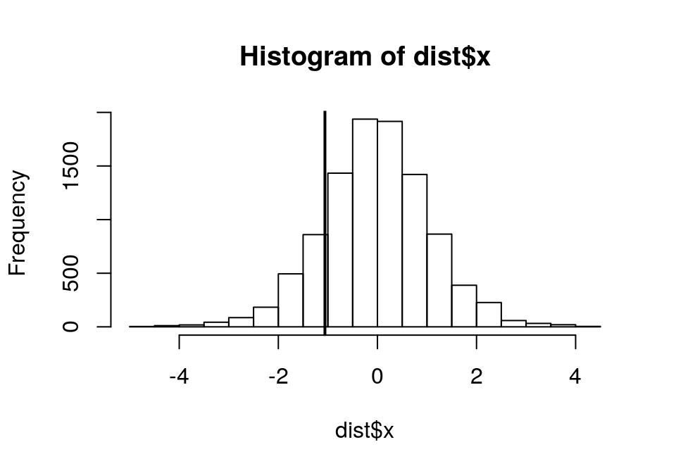
圖 37.1: The sampling distribution of the difference

可以看出來，觀察值的統計量在這10000個新樣本中，並不那麼“極端”。觀察數據的排列置換法 \(p\) 值為：

#Use the distribution to obtain a p-value for the mean-difference by counting how many permuted mean-differences are more extreme than the one we observed in our actual data:
sum(abs(dist) > abs(t.test(dt$thyr ~ dt$group, var.equal = TRUE)$statistic))/10000

## [1] 0.3072

跟下面用參數檢驗法的 \(p\) 值結果做一下對比，就會發現，其實二者的 \(p\) 值結果十分接近。

t.test(dt$thyr ~ dt$group, var.equal = TRUE)

## 
##  Two Sample t-test
## 
## data:  dt$thyr by dt$group
## t = -1.05935, df = 14, p-value = 0.30738
## alternative hypothesis: true difference in means is not equal to 0
## 95 percent confidence interval:
##  -43.256997  14.653823
## sample estimates:
##       mean in group Marked symptoms mean in group Slight or no symptoms 
##                           42.142857                           56.444444

37.3 排列置換法三板斧

標題黨會不服，其實排列置換法的步驟不止三步 (笑)。

在零假設的前提下，確認觀察數據所屬的組別，是可以任意對調的。(exchangeability) 有時候我們可能對數據進行一些轉換 (transforming)，以滿足這個要求。
確認檢驗統計量 \(T\)，用 \(T_{NULL}\) 標記。並且確定零假設時，檢驗統計量的期待值。(通常會用 \(T_{NULL}=0\))
計算觀察數據獲得的統計量 \(T_0\)。
對觀察對象的組別進行 \(N\) 次隨機排列組合。計算每次排列組合情況下的統計量 \((T_1, T_2, \cdots, T_N)\)。
計算 \((T_1, T_2, \cdots, T_N)\) 中比 \(T_0\) 更極端的值所佔的比例 (\(>|T_0|\))，作為觀察值 \(T_0\) 的雙側 \(p\) 值。

37.3.1 該如何選用合適的檢驗統計量 \(T\)？

在排列置換法中選用合適的檢驗統計量是一個需要仔細思考的過程。選用的 \(T\) 必須要能反映組間的差異，並且要與話題相關。也希望能夠盡量和另假設時的統計量有一定的距離\(T_{NULL}\)。然而，選擇了不同的檢驗統計量並不意味著統計結果會有天差地別。最終常常是殊途同歸。另外，檢驗統計量並不一定要是一般參數檢驗時用到的統計量 (\(t\) 或者其他的似然比檢驗)，因為我們不需要對統計量的精確度 (標準差標準誤等統統不要) 作判斷，本法的統計學推斷是通過排列置換的過程實現的。

37.3.2 可以在排列置換法中對其他變量進行統計學調整 (adjustment) 嗎？

用隨機對照試驗做例子。假如在實驗開始前的某個測量變量需要作為共變量被調整 (也就是要用 ANCOVA)，以獲得調整後的 \(Y\) 差異。在零假設條件下，\(Y_i\) 就不滿足可置換原則 (exchangeable)，因為那個需要被調整的測量變量可能決定了他們之間組別是有差異的。

此時，零假設條件 (沒有組間差異) 下，滿足可置換原則的其實是不考慮組別的情況下對需要校正的變量進行線性回歸後獲得的殘差 \(R_i\)：

\[ R_i = Y_i - \hat{Y}_i = Y_i - \hat\alpha - \hat\beta X_i \]

另假設條件下，只有殘差 \(R_i\) 才滿足可置換原則，可以用在排列置換法中。當需要調整的變量個數增加時，同樣適用。

37.3.3 排列置換法，基於秩次的非參數檢驗之間的關係

如果你注意到，當我們把原始觀察數據排序之後進行的排序檢驗其實就是我們本章介紹的排列置換法。它在前面的秩次非參數檢驗中以特殊的形式展現。Good (Good 2006) 曾經說的好，“99% of common non-parametric tests are permutation tests in which the observations have been replaced by ranks. The sign is one notable exception.” 所以符號檢驗是非排序檢驗的特例。

37.3.4 排列置換檢驗法，是一種精確檢驗

複合型假設，指的是假設中只提及了所有分佈情況中的一種的例如：

\[\text{The mean of X is equal to } 0\]

相反，一個簡單假設，則是對參數分佈進行了詳細描述的假設：

\[X\sim N(0,4)\]

所以，對複合型假設進行的統計檢驗法，被稱作精確檢驗法。精確檢驗法的特點是，複合型假設中包含的所有假設發生的概率之和等於該檢驗法的第一類錯誤概率 \(\alpha\)。

A test is said to be exact with respect to a compound hypothesis if the probability of making a type I error is exactly \(\alpha\) for each and every one of the simple hypotheses that are subsumed within the compound hypothesis.

一個大家都聽說過的精確檢驗的例子就是 Fisher 精確檢驗法 (也是一種排列置換檢驗)。所有的排列置換檢驗法都是精確檢驗法。

37.4 基於排序置換檢驗法計算信賴區間

基於排序置換檢驗法的信賴區間計算，是一個有些許繁瑣的過程。我們可以設定多個不同的 \(N_{NULL}\) ，但是樣本分佈相同的零假設時的統計量。計算相應的 \(p\) 值，95% 信賴區間就是 \(p\) 值保持大於等於 \(0.05\)的 \(N_{NULL}\) 取值範圍。計算量將會是很大的。

用前面的例子來解釋就是，我們可以假設兩組之間甲狀腺素的差異是 \(T_{NULL} = 10\)，然後將第二組的觀察值全部加上10 (或者將第一組的觀察值全部減去10)，然後用前面描述的方法來檢驗兩組之間的差是否等於零，獲取 \(p\) 值。然後用不同的 \(T_{NULL}\) 取值，重複這個過程，直到找到上限和下限的 \(T_{NULL}\) 值，他們的檢驗 \(p\) 值都是0.05。

37.5 排序置換法的優缺點

優點：

數據如果大大偏離了參數檢驗法的假設 (完全不是正態分佈)，本法則十分適用，且結果穩健 Robust；
所有的排序置換法計算的 \(p\) 值都是精確不需要近似的；
排序置換法十分可靠，結果不會偏離對應的參數檢驗法，但是當你的數據樣本量很小，無法使用參數檢驗進行理想的統計分析時，排序置換法是極佳的選擇。

缺點：

可置換原則必須得到滿足；
消耗極大的運算能力，當數據量大時，計算過程將會很緩慢；(Windows的話可能直接就死機了，笑)
用排序置換法計算信賴區間的過程比檢驗本身還好耗時費力。

References

Good, P.I. 2006. Permutation, Parametric, and Bootstrap Tests of Hypotheses. Springer Series in Statistics. Springer New York. https://books.google.co.uk/books?id=tQtedCBEgeAC.

第 37 章 排列置換法 Permutation procedures