1 Statistical modelling
1.1 Statistical models
Statistics is about using models to understand data. Statistical models are similar to physical models, such as a map of a city, in that they are simplified but informative representations of our data.
We use statistical models for 3 main reasons:
Description - We use models to describe and communicate our data in a simple way. If I were to conduct a survey of 100 UvA students about how many hours per week they study and I wanted to communicate the results of the study to the UvA administrators, I wouldn’t just send them an excel sheet with 100 responses and say “see!”. To understand and communicate data we need to represent data in a simpler way. The formal way of simplifying data is through statistical modeling. In some cases, the model might be extremely simple. For example, if I tell you that the average student in my survey studied 20 hours per week with a standard deviation of 3 hrs, this already tells you a lot about the 100 data points with just two numbers! While you might not realize it, this is a model! Depending on the data set, we might also want to construct more complex models to describe our data. For example, the hours studied per week might depend on the year of study and the bachelor’s program of the student. In this class, we will learn a flexible framework for modeling our data sets: general linear models.
Inference - We use models to tell us how likely the patterns we see in our data are real patterns vs. due to random chance. In the example above, we wanted to know how much the average UvA student studies, but we only asked 100 students. How can we say something about the general population of all UvA students if we only surveyed a small fraction of these students? What is the risk of coming to the wrong conclusions just by coincidentally asking students that happen to study more or less than usual? We use statistical models to help answer these questions. We can use statistical models to tell us how much uncertainty there is around an observed pattern in our data, or how likely this pattern could result from chance alone.
Prediction - Sometimes variables that are of interest to us are very difficult to measure, and we want to be able to develop models to predict the variable of interest from easier to measure variables. A good example of this comes from remote sensing where images from satellites are used to estimate various variables on earth, for example land surface temperatures, or primary productivity in the ocean. These models are generally developed by fitting collecting datasets where both the variable of interest and the easier to measure variables were measured at various times, and fitting models to find the relationship between the two. These models can then be used to make predictions in cases where the variable of interest was not measured.
1.2 linear models
The basic structure of a statistical model is:
data = model + error
In the equation above, the “model” gives the expected value for any data point, and the error is the difference between expectations and reality. One question then is how should we model our data. In theory, we could use any type of model from complex simulation models to deep neural networks. But in general, we like to keep things as simple as possible. One of the simplest types of models one could use to model data, are linear models.
To illustrate linear models, consider the data below showing carbon emissions of cars as function of their speed:
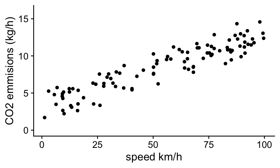
From looking at the data, there appears to be a relationship between CO2 emissions and the speed a car travels. We can model this data, or represent the data in a simpler form, using the equation of a line, or linear equation:
\[ \mathbf{\hat y} = b_0 + b_1 \mathbf{x} \] In the context of this dataset, the predicted value of CO2 is \(\mathbf{\hat y}\) (the hat on top of the y indicates this is a predicted value). On the right hand side of the equation we see that \(\mathbf{\hat y}\) depends on the sum of two terms. The first is \(b_0\) that does not depend on \(\mathbf{x}\) (in our case speed), and the second is a term that increases linearly with \(\mathbf{x}\) (speed). When speed is zero, then our predicted CO2 emission is equal to the value of the \(b_0\), so \(b_0\) is the intercept. In the equation y and x are written in bold because we can think of them as vectors, like columns in an excel file, where each row is a different observation and the length of these vectors is equal to the number of observations in our dataset. This equation provides a way of generating a predicted value of y for each value of x in our dataset.
1.3 Definitions
Dependent variable (y): in the example above the term on the left-hand side of the equation is called the dependent variable, (also: response variable). It is the variable that we model with our statistical model.
Independent variables (x): In statistical models, we model the dependent variable as a function of independent variables (also: predictor variables). We use the term independent variable because the dependent variable depends on the values of the independent variables, or the response variable depends on the value of the predictor variables.
Parameters (intercept (\(b_0\)) and slope (\(b_1\))): The parameters determine the exact relationship between the dependent variable and the independent variables. In the example above, the intercept determines the modeled value of CO2 emissions for an idling car, and the slope parameter determines how much the modeled CO2 value increases per unit increase in speed.
Problem 1.1 In the next section, we will learn how to precisely fit models to data, but you should be able to look at the plot and get a rough estimate of what the model parameters need to be for the model predictions to approximate the data. Before moving on look at the figure above and estimate the two parameters of the statistical model.
In this case, the \(b_0\), the intercept is very easy to estimate. The observations for cars with speeds close to zero have \(CO_2\) emissions around 3 kg/h. For \(b_1\), the slope, we can see that typical emissions go from around 3 to 13 kg/hr as we go from 0 to 100 km/hr. Thus the slope of this relationship is (13-3)/(100-0) ~ 0.1 (kg/hr)/(km/h).
If we then plot out the equation:
\[\hat y = 3 + 0.1 x\]
we see that this simple linear model does a good job at capturing the trend in the data:
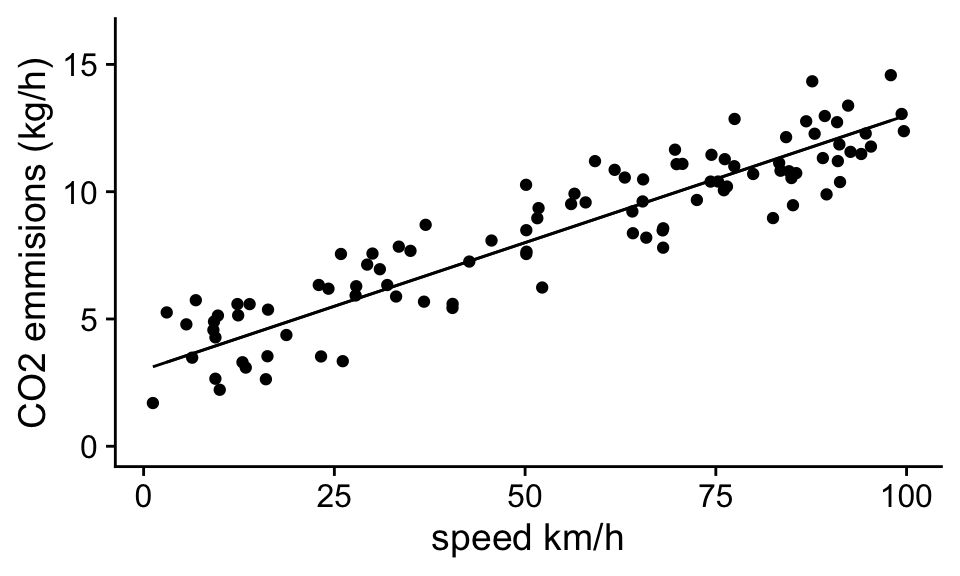
Importantly by using a model to describe our data, we are able to boil 100 observations down to 2 numbers, a slope and an intercept that capture the salient features of the data. This allows us to convey important information about the data, for example, how quickly does CO2 emissions go up with speed, or how much CO2 does the average idling car emit? It is important to note that there is variability in the data set, different cars have different CO2 emissions even when traveling at the same speed. This has several consequences.
1. Statistical models are not perfect representations of our data, for any observation there will be some deviation between the predicted and the observed value. This is related to the equation we first introduced: data = model + error. In our new notation the data is \(y\), the model predictions are \(\hat y\), and the difference between observations and model predictions is the error.
\[data = model + error\] \[y = \hat y + error\] In the context of an entire dataset, we have a vector (column) of values for the variable, predictions and errors: \[\mathbf{y} = \mathbf{\hat y} + \mathbf{error}\]
2. Parameter estimates of our model in part depend on which random sample we collected in our study. If we repeated our study with a different random set of cars we would probably get a slightly different result. This is an important and general problem with data and one that we will use statistical models to help solve in chapter 3 (Uncertainty).
1.4 Categorical independent variables
In the example above the independent variable (speed) was continuous. But independent variables can also be categorical, for example, we might want to know carbon emission of cars vs trucks.
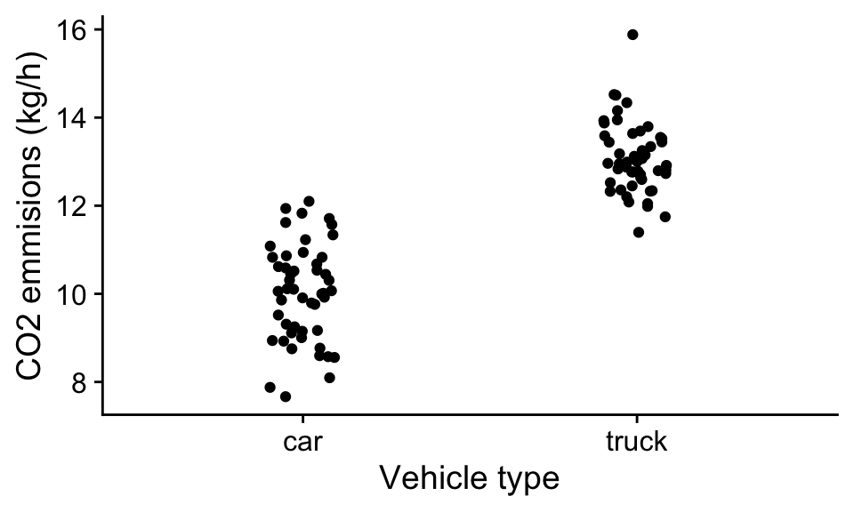
Here we have two classes of the independent variable that don’t fall on a continuous scale. However, we can use the same linear model framework with categorical variables:
\[\mathbf{\hat y} =b_0 + b_1\mathbf{x}\] but now, each value in the vector \(\mathbf{x}\) equals either a 1 or 0 depending on the class of the independent variable. For example, if the vehicle is a car, x = 0, and if it is a truck x = 1.
This means our predicted CO2 emission for cars would be: \[\hat y =b_0 \] And for trucks would be: \[\hat y =b_0 + b_1\] Thus the parameters of our linear model have clear interpretations. The \(b_0\) is the expected CO2 emissions for cars, and the \(b_1\) parameter is the expected difference in emissions between trucks and cars. We would expect the \(b_1\) parameter to be positive if trucks have higher emissions than cars.
It might seem arbitrary which class of a categorical variable is set to 0 and which is set to 1, and in fact it is, but either way results in the same interpretation.
Problem 1.2 Prove to yourself that the order of the dummy variables doesn’t affect your interpretation of the result. By eye, estimate the parameters of the model for both possible orderings of the dummy variables (Case 1: x = 0 if car, x= 1 if truck; Case 2: x = 1 if car, x = 0 if truck).
You should have found that the magnitude of \(b_1\) is the same in both cases, but that the sign depends on the ordering. In the first case, when x = 0 if the vehicle is a car, then \(b_1\) is the estimated change in CO2 emissions if we switch from a car to a truck (\(b_1\) is positive). And in the second case, (x=1 if the vehicle is a car), \(b_1\) is the estimated change in CO2 emissions of switching from a truck to a car (\(b_1\) is negative). In practice R will automatically assign dummy variables to categorical independent variables (based on alphabetical order). In some cases, specific orderings of the variables are more logical. For example, in an experiment we might want adopt x=0 for the control and x=1 for the treatment. You can override the default ordering of levels in R to change this if desired.
1.5 More than two classes of catagorical variables
If we have more than two classes of an independent variable, for example, cars, trucks, and motorcycles, then we need to introduce more dummy variables:
\[\mathbf{\hat y} = b_0 + b_1 \mathbf{x_1} + b_2 \mathbf{x_2}\]
In this formula, \(\mathbf{x_1}\) and \(\mathbf{x_2}\) are column vectors of 0’s and 1’s where the value of each row depends on the type of vehicle. For example, we could set \(x_1\) equal to 1 if the vehicle is a truck and equal to 0 if not. Similarly, we can set \(x_2\) equal to 1 if the vehicle is a motorcycle and 0 if not.
Problem 1.3 Assume that \(x_1 = 1\) indicates a vehicle is a truck and \(x_1 = 0\) that it is not and \(x_2 = 1\) indicates a vehicle is a motorcycle and \(x_2 = 0\) that it is not. What is then the interpretation of each of the parameters in the model?
For cars \(x_1\) and \(x_2\) will both equal 0 so the expected CO2 emission will equal \(b_0\). For trucks \(x_1\) = 1 and \(x_2\) = 0 so \(b_1\) is the expected difference between truck emissions and car emissions (which will be positive if trucks emit more CO2 than cars). For motorcycles \(x_1 = 0\) and \(x_2 = 1\) so \(b_2\) is the expected difference between motorcycle emissions and car emissions (which will be negative if motorcycles emit less CO2 than cars).
1.6 Interpreting parameters
Throughout the course, and later on in your career, you will fit statistical models to data, and then need to interpret and communicate your findings to colleagues, stakeholders, or the public. You often hear the parameters in a linear model being referred to as “effects”. For example, in the vehicle emissions example, you might say that the “effect” of vehicle type was 2, or the effect of speed on emissions was 0.1. The word “effect” is tempting to use (and I am sure I will accidentally use it during the course) because it is an easy shorthand for describe the model results. However, the problem with the work “effect” is that it implies the independent variable causally affects the dependent variable. This is related to the idea that correlation is not causation. Just because we find a linear relationship between the dependent variable and the independent variable it does not indicate causation. If you need to be convinced of this statement, I highly recommend you check out the website: https://www.tylervigen.com/spurious-correlations
The safest way to interpret parameters in a statistical model is comparisons. For example, in CO2 emissions example, we can interpret the value of the parameter \(b_1\), associated with vehicle type, as the estimated average difference in CO2 emissions of trucks compared to cars, which was roughly 2 kg CO2/hr.. And for \(b_2\), the average difference in CO2 emissions of vehicles of the same type, but differing in speed by 1 km/hr is approximately 0.1 kg/hr. As you can see, it is a bit more awkward to describe model parameters as comparisons rather than effects, and in the case of CO2 emissions, the causal links between vehicle type and speed with CO2 emissions is straightforward, but it many cases this won’t be true. For example in many observational studies, if you find an association between two variables, it could be due to a causal link, but it could also be because the independent variable is correlated with another variable that is causally affects the dependent variable. If we use language like the “effect of x” in these cases gives the impression that it we experimentally manipulated x, it should the effect on y predicted by the linear model, which will not always be the case.
The only time it is relatively safe to use causal language to describe parameters in statistical models is in the context of randomized experiments. In this case, if the experiment was designed appropriately, there should be on average no systematic differences between individuals except for the treatment assignment, which allows us to rule out other potential causal mechanisms. You could still observe differences between treatments in an experiment due to chance, but we can use statistical methods to quantify this risk.
1.7 More complex models
The generality of general linear models comes from the fact that we can add as many independent variables to the model as we want.
For example, we could model CO2 emissions as a function of both car type and speed:
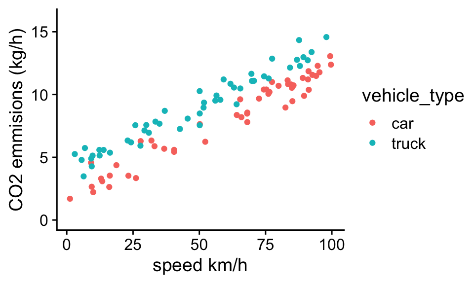
Problem 1.4 Think about what type of simple model you could use to model the data that accounts for the effect of vehicle type and speed on carbon emissions. Write down the model as a linear equation and define all independent variables and parameters. By eye, estimate roughly what the parameters of this model should be to fit the data.
Looking at the data, we can see again the clear trend of vehicle type and speed on CO2 emissions. For a given speed, trucks have higher emissions than cars, and for both cars and trucks emissions increase with speed at roughly the same rate. We can account for these two factors in the model:
\[\mathbf{\hat y}= b_0 + b_1 \mathbf{x_1} + b_2 \mathbf{x_2}\]
where
\(x_1\) is a dummy variable that equals 0 if the vehicle is a car and 1 if it is a truck
\(x_2\) is the speed of the vehicle
\(b_0\) is the expected C02 emissions for a stationary car (roughly 2 kg /hr)
\(b_1\) is expected difference in emissions for trucks over cars (roughly 2-3 kg /hr)
\(b_2\) is the expected C02 emission for a stationary car (roughly 0.1 [kg/hr]/[km/h])
Note in this case we assumed that the effect of speed on emissions was the same for cars and trucks. This may not always be the case. Later in the class we will learn how to deal with cases where the effect of one independent variable depends on the value of another independent variable.
For each new independent variable included in our model, we will need a new parameter that relates the value of the independent variable to its effect on the expected value of the dependent variable.
1.8 What makes a linear model “linear”?
Linear models have the general framework:
\[\mathbf{prediction} = intercept + parameter_1 * \mathbf{variable_1} + … + parameter_n * \mathbf{variable_n} \] or: \[\mathbf{\hat y} = b_0 + b_1 \mathbf{x_1} + … + b_n \mathbf{ x_n}\] The model is linear in the sense that the predicted values of the model is a linear combination of the independent variables:
\[\mathbf{\hat y} = b_0 + \sum b_i \mathbf{x_i}\]
Linear in the context of linear statistical models means linear in the parameters, such that the change in \({\hat y}\) due to a change in the parameters does not depend on the value of the parameters. Thus if \(\frac{d \hat y}{db_i}\) does not depend on the value of \(b_i\) for all of the parameters then the model can be written down as a linear statistical model.
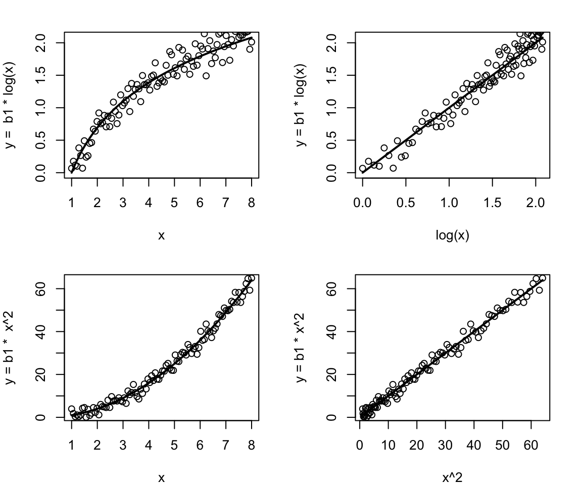
The fact that a given change in the value of a model parameter results in the a same change in \(\hat y\) regardless of the value of the parameters makes it possible to analytically solve for the parameters that best fit the data. More advanced and computationally expensive methods are needed to fit non-linear to data, and in general, there is no guarantee that we will find the parameters that best fit the data. Fortunately, linear models are not quite as restrictive as you might think. This is because we can transform or combine independent variables in whatever what we see fit and still have a ‘linear’ model. For example, we could log transform an independent variable:
\[\hat y = b_0 + b_1 \log(x)\] or square an independent variable:
\[\hat y = b_0 + b_1 x^2\] and still have a linear model. We can think of \(\log(x)\) or \(x^2\) as new independent variables, and the predicted value of y is just a linear combination of the new independent variables (right panels). In this way, linear models can fit data that don’t look linear (left panels).
Examples of non-linear models would be
\[\hat y = b_0 + x^{b_1}\]
or
\[\hat y = x_1 / (b+ x_1)\] An easy way to tell if a term in a model is linear is if you can arrange the term so that you have the parameter times any combination or transformation of independent variables. For example the term:
\[ \frac{ b_0 x_1 }{x_2+ x_1}\] is linear because we can put parentheses around everything but the parameter:
\[ b_0 \left( \frac{ x_1 }{x_2+ x_1}\right)\] We can think of everything inside the parentheses as a new independent variable: \[ b_0 x_{new}\] where \[ x_{new}=\left( \frac{ x_1 }{x_2+ x_1}\right)\]
Problem 1.5: Which of the following models can be made linear by substitutions? The “b”s are parameters and “x”s are independent variables.
\(\hat y = b x^2\)
\(\hat y = b \sin(x)\)
\(\hat y = \sin (b x)\)
\(\hat y =b_0 \sin (b_1 x)\)
\(\hat y = b x_1 x_2\)
\(\hat y = b x_1 ^ {x_2}\)
\(\hat y = \frac{ x_1} b\)
\(\hat y = b \log(x_1 x_2)\)
Answers: 1 Yes, 2 Yes, 3 No, 4 No, 5 Yes, 6 Yes, 7 No, 8 Yes
1.9 General linear models
As introduced above, we will be using linear models to model the relationship between independent variables and dependent variables. More specifically, we will be working with a class of statistical models refered to as General Linear Models. In the equation:
data = model + error
General linear models models, assume that the “model” term is composed of linear relationships between independent and dependent variables as descibed above, but it also assumes that the errors are normally distributed. More specifically it assumes that
error ~ N(0,\(\sigma\))
which means that the errors are drawn from a normal distribution with a mean equal to zero and a standard deviation equal to sigma. In many cases when the dependent variable is continuous (e.g. carbon emissions, blood pressure, height, weight, precipitation, ect.), a normal distribution is a decent approximation for the distribution of the errors. In Chapter 3, we discover why normal distributions tend to show up so frequently with continuous data.
1.10 Assumptions of General Linear Models
There are 4 main assumptions when we use general linear models.
1.10.1 Linearity
General linear models assume that the relationship between dependent and independent variables is linear. For example, in the plot below, the relationship between x and y is not linear, and thus when we fit a linear model, the predictions of the model are systematically biased in a way that depends on the value of x.
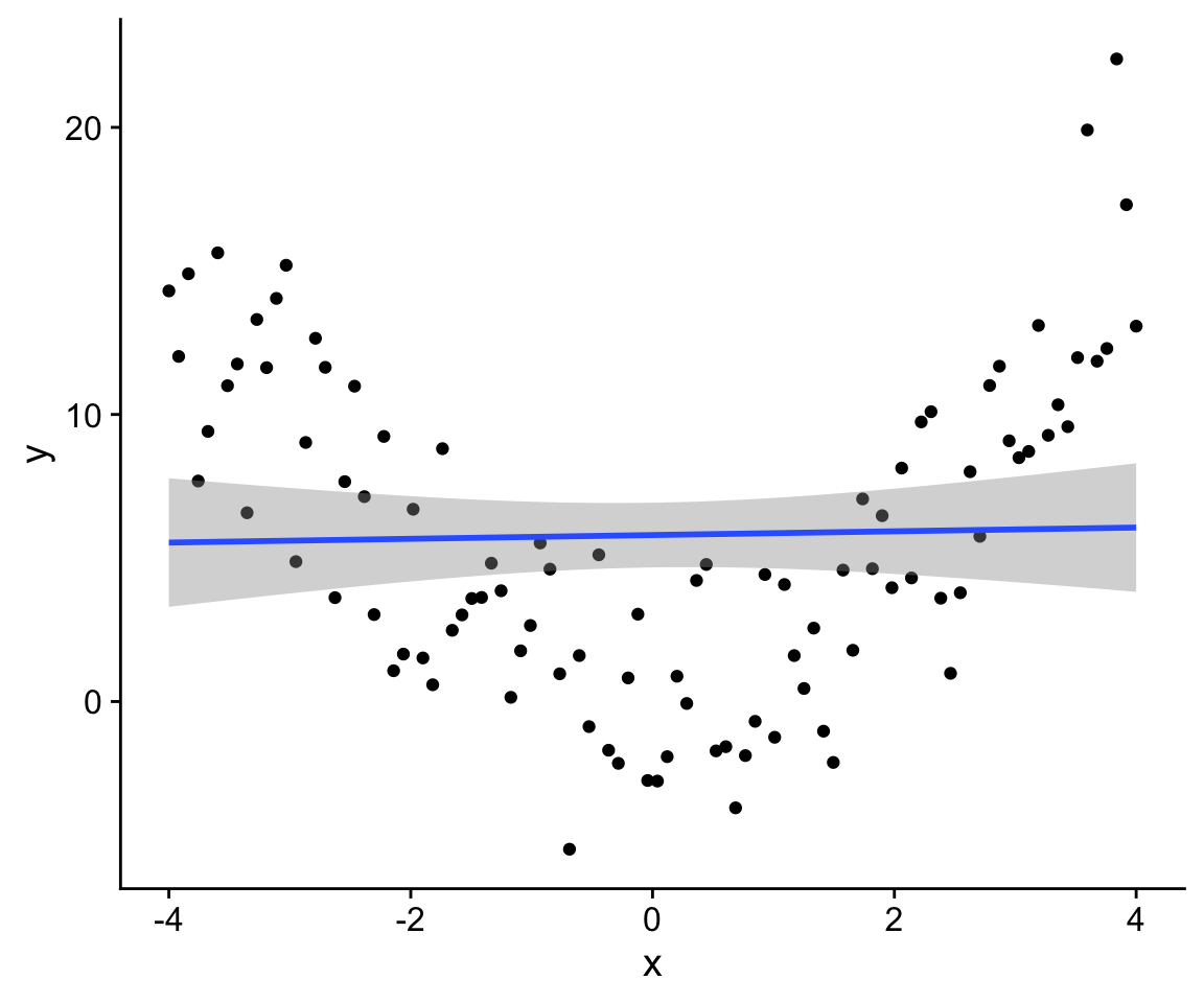 In this particular case, we might estimate the slope of the linear relationship to be very close to zero. In a way, this inference is still correct; however, at the same time, this statistical model doesn’t really capture the relationship between x and y. By fitting a more complex model, we can see that there is a relationship between x and y, it is just not linear.
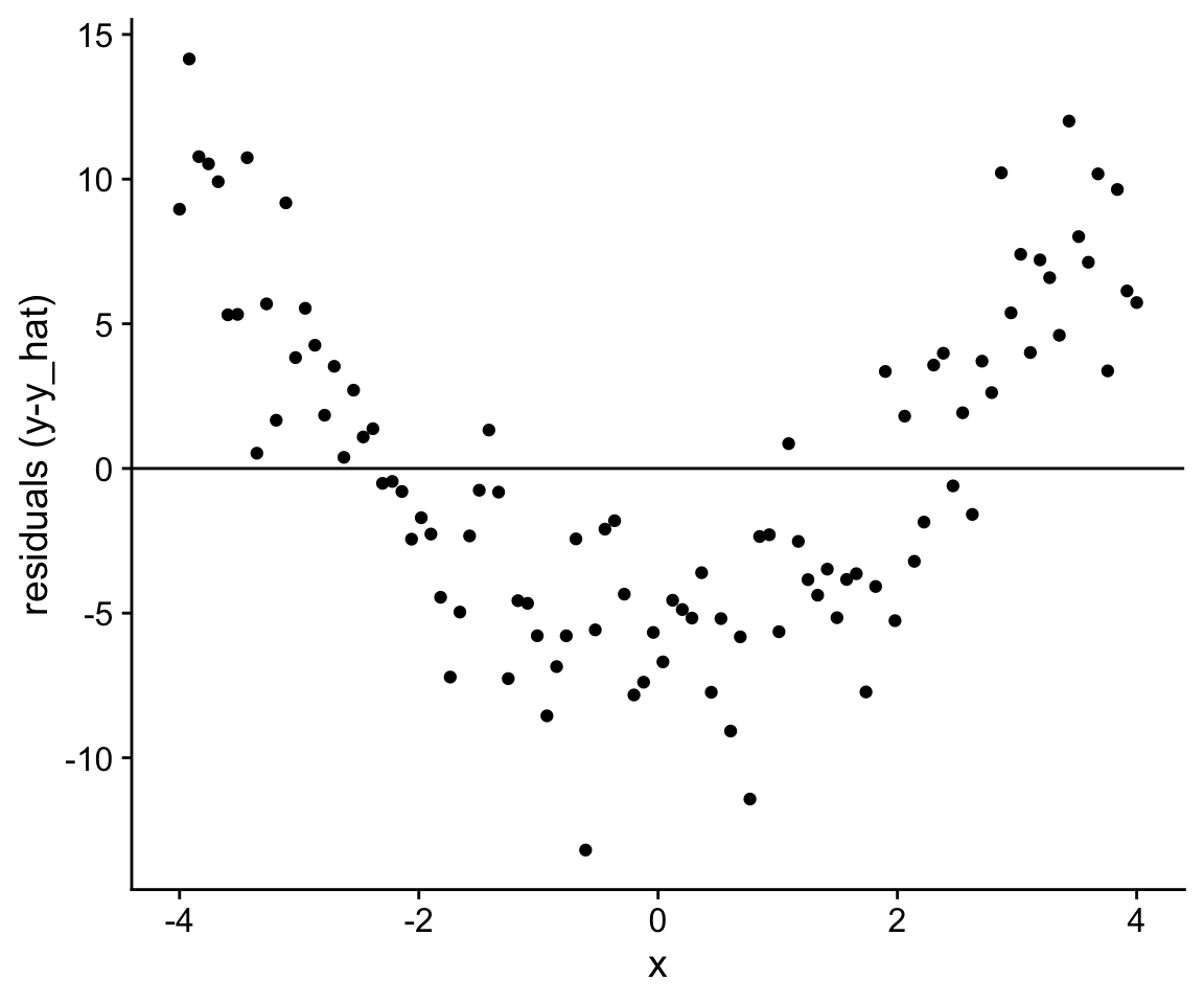
Extreme violations of the linearity assumption can often be revealed by plotting the model prediction along with the data. If the residuals, or differences between observations and predictions, differ systematically as a function of the independent variable, this is a good sign that the wrong model is being used for the data at hand.
Later in the course, we will discuss how more complex (but still linear) models or data transformations can be used to avoid substantial violations of the linearity assumption.
1.10.2 Normality
General Linear Models assume that errors (or residuals) are normally distributed. Thus if you were to plot a histogram of the model residuals, you would expect to see a distribution that is centered around zero, and roughly symmetric:
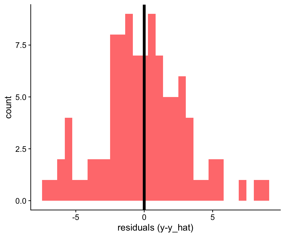
In other cases, our residuals might look heavily skewed:
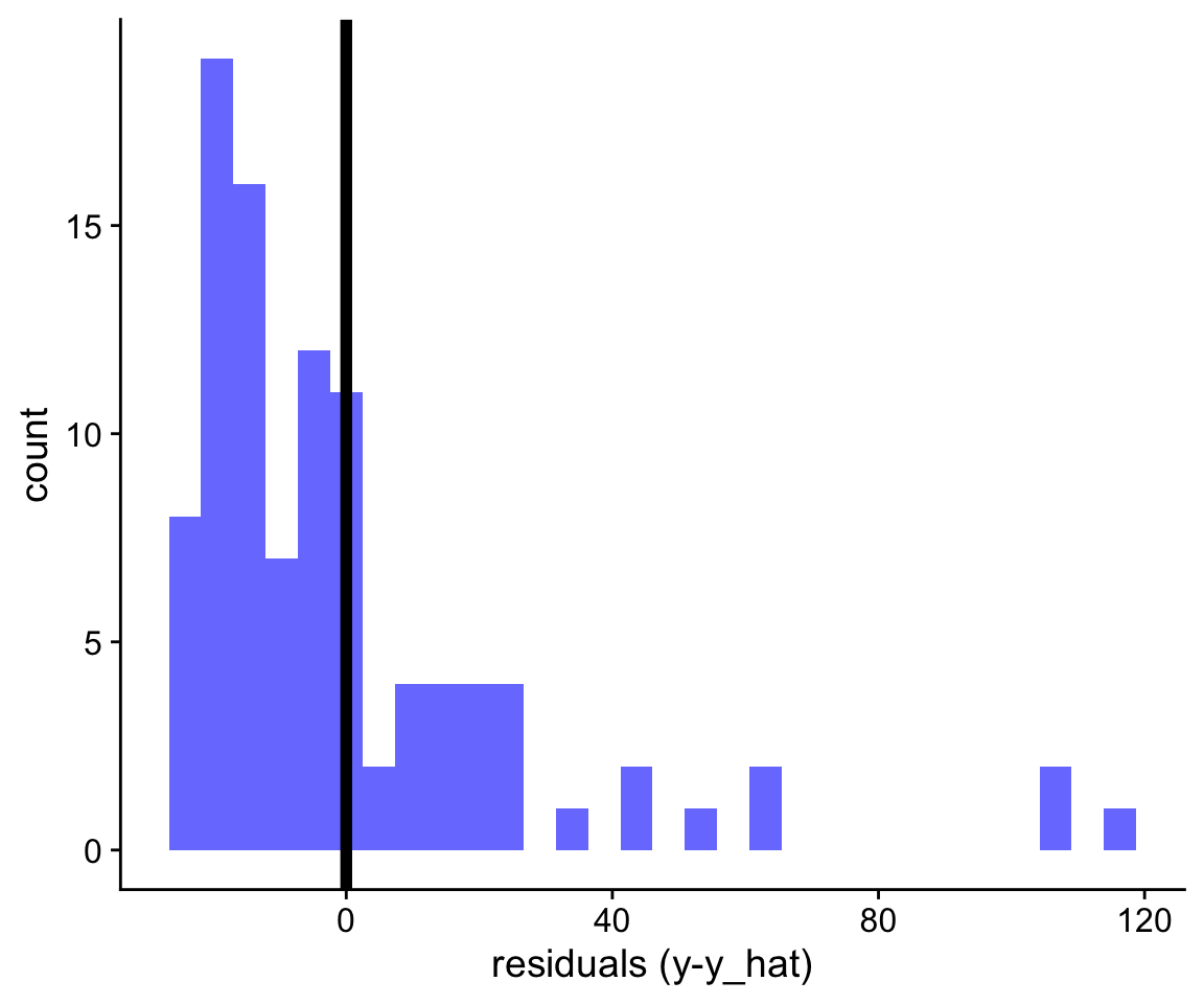 As we will see later in the course, even when residuals are clearly not normally distributed like in the example above, the statistical inferences are often still valid. However the main problem with the example above is that the means don’t really reflect an “average” or typical value because most observations have values below the mean. In cases like this, sometimes transforming the data, for example, using log(y) rather than y as the dependent variable allows the mean to better capture the central tendency of the data.
1.10.3 Constant variance
As stated earlier, general linear models assume errors are drawn from a normal distribution with a mean of zero and a standard deviation of sigma, where \(\sigma\) is a specific value for a given dataset:
error ~ N(0,\(\sigma\))
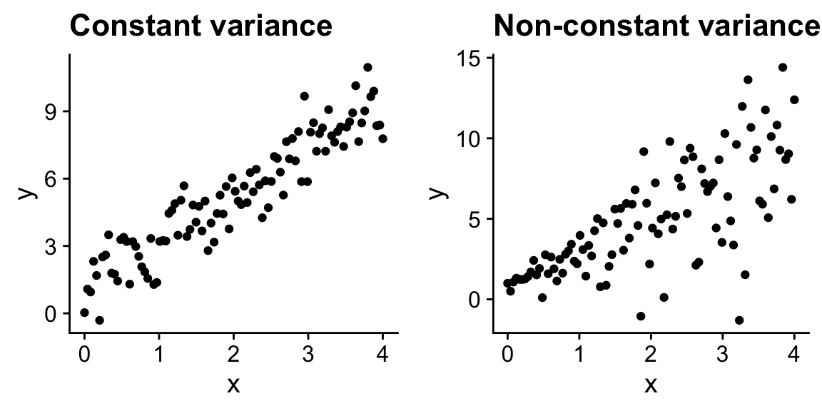
Because \(\sigma\) is a fixed value, this means that our model assumes that the variance doesn’t systematically change with as a function of the independent or dependent variables. In the figure below, on the left is an example where the variance appear to be constant across the range of x values, and on the right is an example, where the variance appears to increase with x. Thus in the figure on the right, the constant variance assumption is not met. Again, like for the normality assumption, it turns out that the results from general linear models are fairly robust to violations of this assumption.
1.10.4 Independence
General linear models assume that to independent of other errors. This is by far the most important assumption, and even small violations can have important implications.
Consider an example where a pollster randomly samples 1000 households to gauge political preferences. However, to increase their sample size, the pollster decided to not only poll the randomly selected individual, but also their partner. As a result the pollster end up with nearly double their originally planned sample size, and thus was able to get more precise statistical estimates of political preferences.
Can you think of a problem here?
The problem is that the statistical model is based on the assumption that we have 2000 independent data points, but in all likelihood, individuals are likely to share the political preferences of their partners, and thus the political preference of one individual is not independent of their partner’s preferences. In the most extreme case, if people only partnered with individuals with identical political preferences, then there is no new information gained by asking partners about political preferences. In this case, even though the pollster asked 2000 individuals, they effectively only have 1000 true observations, and thus their analysis based on 2000 individuals will drastically overestimate our certainty about estimates of political preferences.
Non-independence of errors shows up in many contexts. For example observations might be correlated because they were taken from locations that are close in space or time, or observations taken from the same individual multiple times. In some cases non-independence of errors is inevitable, and thus we have to use more advanced statistical approaches that account for dependencies (for example, time-series analysis or spatial statistics). However, when possible it is best to design experiments of field studies to avoid dependent errors through randomization.
1.11 What you should know
1. The general structure of linear models, including distinguishing parameters, independent variables, and dependent variables
2. Be able to write general linear models to describe simple data sets with both continuous and categorical independent variables, and interpret the meaning of each parameter and variable in the model.
3. Be able to roughly estimate parameter values of simple linear models by looking at a figure (e.g. problem 1.1 and 1.4)
4. Be able to tell whether a statistical model is linear (e.g. problem 1.5)
5. The assumptions of general linear models