4 Hypothesis testing
4.1 Recap
In part 1, we learned how to formulate linear models to model data. In part 2, we learned how these models are fit to data, and various ways to quantify goodness of fit. In part 3, we learned how to quantify the uncertainty about the true value of the parameters in our model given a particular dataset. In a way, if you understand these three chapters well, you are already prepared to begin using models to learn from data. In part 4, we will cover how we can use models to test (null) hypotheses.
Null hypotheses significance testing (NHST), p-values, and the concept of “statistical significance” are frequently used and abused by scientists and the media. In fact, there is an ongoing debate in science about whether and when NHST should be used at all. Some journals have even gone so far as to ban the use of NHST! You have already come across NHST in previous stats classes, but if your like many practicing scientists, there is a good chance you don’t quite understand how to use and interpret the results of NHST correctly. The goal of this chapter is to demystify p-values, statistical significance, and null hypothesis testing, so that you can better understand your own statistical results, but also be able to critically assess statistical results reported in scientific papers and the media.
4.2 The motivation behind p-values
Let’s say you conducted a study to test whether a drug can reduce blood pressure, and you found that on average people who took the drug had lower blood pressure compared to those who took a placebo. You are excited about the result, but then you begin to worry: what if this result is just a coincidence? For example, if the drug truly had no effect, there would be a 50% chance of observing lower average blood pressures in the drug group (the chance that they are exactly the same on average is vanishing small). This is the problem that p-values a meant to help deal with. A p-value is the probability of observing the effect we observed (or a larger one) due to chance alone. By “effect” I mean the magnitude of a parameter value in a statistical model. If p is close to 1, it means that we should expect to see effects (a parameter estimate) as or more extreme than the one observed in out study quite often due to random chance alone. If the p-value is very low it means that we would expect to see the type of results we observed due to random chance only rarely.
A common statistical practice is to formulate a null hypothesis, which generally corresponds to there being no effect of an independent variable (parameter = 0). In the blood pressure example, a null hypothesis would correspond there being no true average difference in blood pressure between people receiving the drug vs. a placebo. So in the linear model:
\[\hat y =b_0 + b_1x\] \(x_1 = 0\) if placebo, and \(x_1 = 1\) if drug. Then \(b_1\) is the estimated difference in blood pressure between those receiving the drug, vs. a control. The null hypothesis in this case would be \(b_1=0\). If the null hypothesis is true, then any difference we observed between individuals on the drug. vs. placebo is due to random chance. We calculate the probability of observing the difference we observed in our study (or a larger difference) with the p-value.
4.3 Convensional use of NHST
The ‘test’ part of the null hypothesis significance tests, and probably the most controversial part, is a using p-value to come to a binary interpretation of the results (reject the null hypothesis or accept the null hypothesis). If a p-value is below some threshold, one rejects the null hypothesis. Essentially this means if the probability of observing the parameter estimate observed in the study is very low when the null hypothesis is true, the null hypothesis is rejected. This threshold, commonely refered to as alpha, is called the false positive rate. By convention, in biology and many other disciplines, alpha is generally set to 0.05. In this case, the null hypothesis is rejected when the p-value is below 0.05. In other words, we reject the null hypothesis when there is less than a 5% chance of observing a parameter value as or more extreme than the value estimated in our study if the null hypothesis is true. We call it a false positive rate, because if the null hypothesis is true, we would still reject the null hypotheses 5% of the time. If the p-value is greater than alpha, then we fail to reject the null hypothesis. By convention, results with a p-value less than 0.05 are considered “statistically significant” and those with a p-value greater than 0.05 are considered ‘non-significant’.
4.4 P-values and NHST: an example
To get a better idea of how p-values are calculated, let’s work through an example with data from the blood pressure study. The study had 100 participants, with 50 randomly assigned the drug, and 50 assigned the placebo. In this case the null hypothesis was that there is that there is no true difference between control and drug groups. So in the statistical model this is equivalent to \(b_1=0\). They also decided that the will reject the null hypothesis if the probability of observing \(b_1\) as or more extreme than the value measured in their study due to chance is less than 5.
The researchers collected the following data, where ‘bp_change’ was the change in blood pressure during the study, with negative values indicating a reduction in blood pressure.
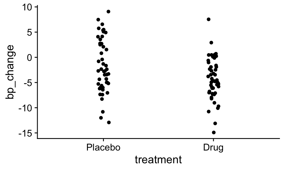
In the plot above you can see that on average, patients that received the drug experienced a lower drop in blood pressure than those that received a control. But the question, is how likely would this extreme of a difference emerge just due to random chance when there were no true differences in the effectiveness of the drug over the placebo.
We can begin to answet his question by fitting our linear model, and calculating the parameter estimates and their standard errors.
mod<-lm(bp_change~treatment,df)
summary(mod)
Call:
lm(formula = bp_change ~ treatment, data = df)

Residuals:
     Min       1Q   Median       3Q      Max
-11.2445  -3.0409  -0.6127   3.7715  11.9445

Coefficients:
              Estimate Std. Error t value Pr(>|t|)
(Intercept)    -1.6753     0.6714  -2.495  0.01426 *
treatmentDrug  -2.7330     0.9495  -2.878  0.00491 **
---
Signif. codes:  0 '***' 0.001 '**' 0.01 '*' 0.05 '.' 0.1 ' ' 1

Residual standard error: 4.747 on 98 degrees of freedom
Multiple R-squared:  0.07795,   Adjusted R-squared:  0.06854
F-statistic: 8.285 on 1 and 98 DF,  p-value: 0.004908
Problem 4.1 We see two rows in the coefficients tables. Which parameters do each of these rows correspond to in the linear model. What is the interpretation of each parameter? Which of these rows is most relevant for testing our null hypothesis that the drug has no effect relative to a placebo?
Hopefully it should be clear to you that the first row, corresponds to the intercept in the linear model, b0, which in this case is the estimated change in blood pressure for patients recieving the placebo. The second row corresponds to the estimated difference in the change in bp for individuals receiving the drug vs, the placebo. The null hypothesis pertains to the 2nd row in the data set, where the null hypothesis is that this parameter is 0.
By looking at the second row, we see that patients that took the drug had on average a 2.73 greater reduction in blood pressure than the control group. We can also see that the standard error for this parameter is 0.9495. We can use these values to calculate the range of parameter values of b_1 that are consistent with the data:
b1 = seq(-8,6,length.out=100)
pdf = dnorm(b1,summary(mod)$coefficients[2,1],summary(mod)$coefficients[2,2])
plot(b1,pdf,'l',ylab='density')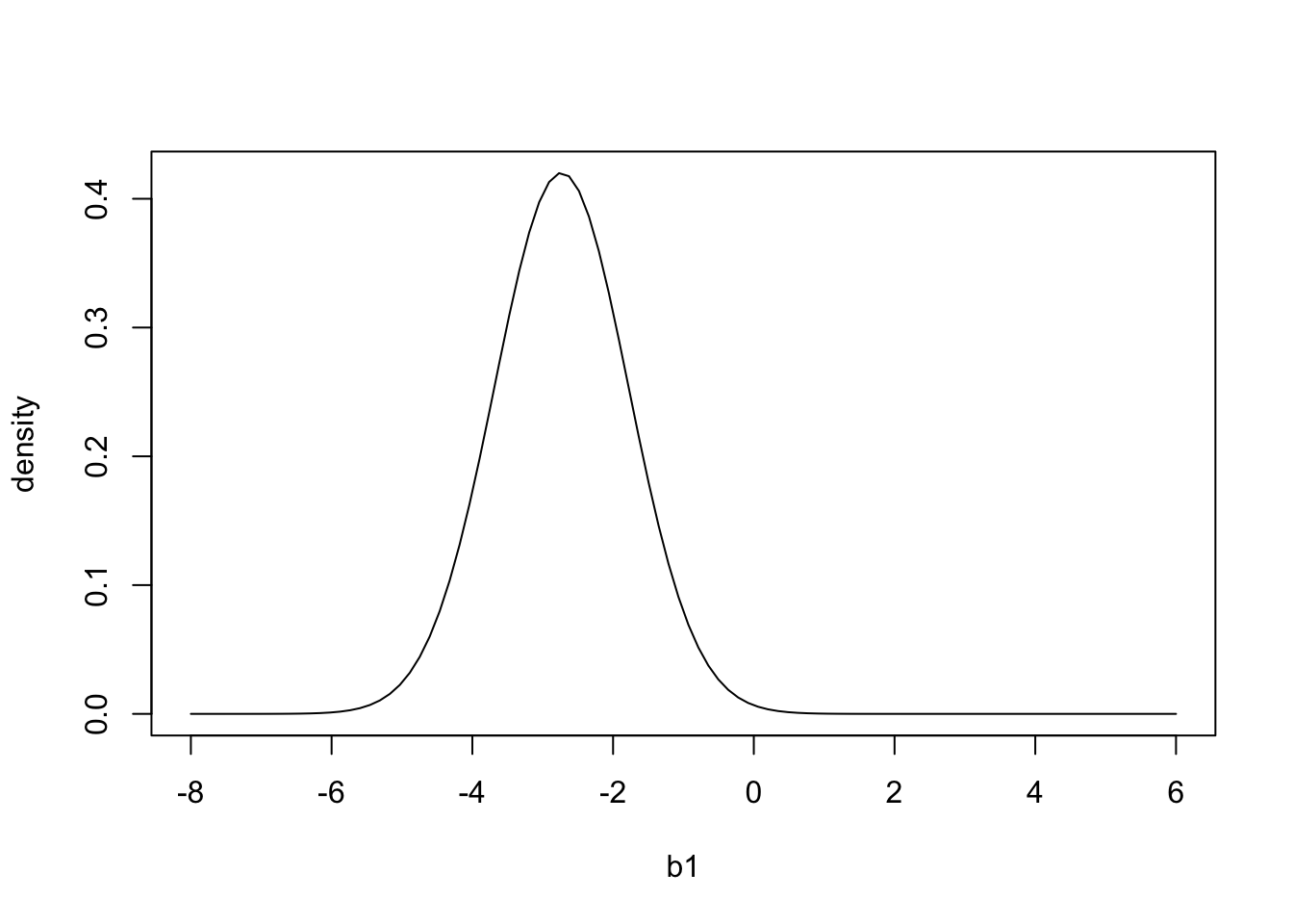 And if we wanted to 95% calculate confidence intervals for \(b_1\), using both the 2 SE method and the more exact way:
# 2SE method
lower_CI_2SEmethod <- summary(mod)$coefficients[2,1] - 2 * summary(mod)$coefficients[2,2]
upper_CI_2SEmethod <- summary(mod)$coefficients[2,1] + 2 * summary(mod)$coefficients[2,2]
# more precise method
deg_free = 98 # 100 data points - 2 parameters
crit_value <- qt(0.975,deg_free)
lower_CI_exact<- summary(mod)$coefficients[2,1] - crit_value * summary(mod)$coefficients[2,2]
upper_CI_exact <- summary(mod)$coefficients[2,1] + crit_value * summary(mod)$coefficients[2,2]
plot(b1,pdf,'l')
abline(v=lower_CI_2SEmethod,col='red')
abline(v=upper_CI_2SEmethod,col='red')
abline(v=lower_CI_exact,col='blue',lt='dashed')
abline(v=upper_CI_exact,col='blue',lt='dashed')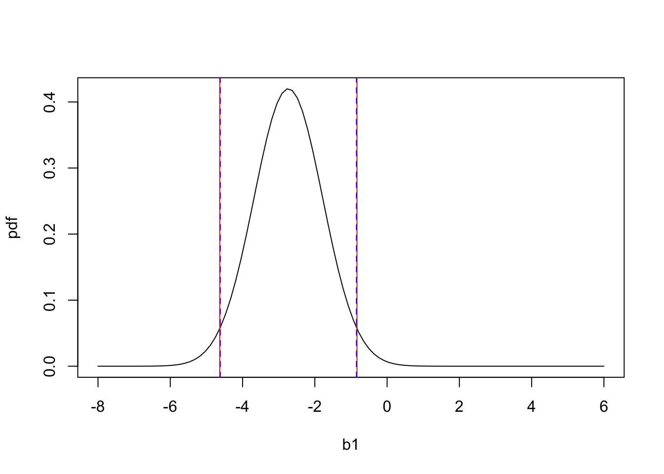 We see first, that the 2 SE method (red) is a very close approximation of the exact method (blue) for calculating 95% confidence intervals. We also see that the 95% confidence intervals do not include 0. Thus we can be 95% confident that the true population is between -4.62 and -0.85, and this range does not include the null hypothesis. This actually already tells us that we will reject the null hypothesis, with an alpha of 0.05. But below we will go through and show how to calculate the p-value.
So we have estimated our parameter of interest it’s uncertainty (standard error). The logic of null hypothesis testing is then to say, lets assume for a moment the null hypothesis is true \(b_1=0\). Given how much uncertainty there is in the parameter value (determined by its standard error) how likely would it have been to observe a \(b_1\) as far or further from zero than the one we observed. You can think of this, as taking the estimated probability density function in the figure above and centering it on 0, which is like assuming \(b_1 = 0\). In the plot below we see the expected sampling distribution of \(b_1\) under the null hypothesis. We can then compare this distribution to to observed \(b_1\) value in our study (vertical line):
b1 = seq(-8,6,length.out=20000)
est= summary(mod)$coefficients[2,1]
pdf = dnorm(b1,0,summary(mod)$coefficients[2,2])

plot(b1 ,pdf,'l',xlab='b1',ylab='density')
lines(b1,b1*0)
abline(v=summary(mod)$coefficients[2,1])
polygon(c(b1[b1<=est],est), c(pdf[b1<=est],0), col=alpha("red",.5))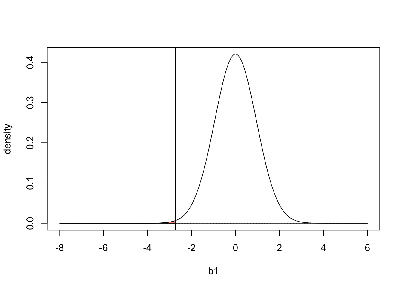
The the area of the red shaded region in the plot above corresponds to the probability of observing a \(b_1\) value less than the value measured in our study if the null hypothesis is true (\(b_1=0\)). Or in other words, how likely is it to have observed a difference in the reduction of blood pressure between the drug and placebo group of -2.73 or less due to random chance alone.
We can calculate this value with the pnorm() function, which is just the are under the curve in the plot above up to the observed value of \(b_1\).
estimate = summary(mod)$coefficients[2,1]
se = summary(mod)$coefficients[2,2]
pnorm(estimate,0,se)
[1] 0.0019987944.5 One-tailed and two-tailed tests
Thus the probability of observing a value of \(b_1\) in the study of -2.73 or less is 0.002. This would be the p-value for what is know as a one tailed test null hypothesis test.
A confusing convention with p-values is that they primarily are used as the probability of seeing parameter value being as least as “extreme” (different from zero) as the observed value if the null hypothesis is true. This means we need to account for the probability of observing \(b_1\) being less than -2.73 and also the probability of it being greater than 2.73. Because the normal distribution symmetric, the probability of \(b_1\) being more extreme than our estimate \(b_1\) > abs(estimate) is 2 times the probability of \(b_1\) < estimate.
So the p-value for a 2 tailed test would be:
2 * pnorm(estimate,0,se)[1] 0.003997588This is referred to as a two-tailed test, because we are accounting for probability of observing a \(b_1\) more extreme (further from zero) than the one observed in our study due to random chance. By convention, we mostly use two-tailed tests because they are more conservative (it is harder to reject the null hypothesis). This is despite the fact our hypotheses are often directional. For example in the case of the drug, we are really only interested in the case where it improves blood pressure relative to a placebo, not in cases where it makes patients worse, so it might make more sense to use a one tailed test. However, by convention, most researchers use a 2 tailed and an alpha of 0.05.
You might notice that the p-value we calculated is slightly different than the value reported in the lm() summary table. This small discrepancy is because we used the normal distribution to calculate the probability of observing a more extreme value of \(b_1\), but the more precise way is to use the t-distribution to account for uncertainty in the standard error of the parameter estimate. To calculate the p-value more precisely, we just take parameter estimate and divide by its standard error, which gives us a t-value:
summary(mod)$coefficients[2,1]/summary(mod)$coefficients[2,2][1] -2.878352which tells us how many standard errors the estimated parameter value is from zero. We can then calculate the probability of observing a value less than this if the null hypothesis is true using pt() (similar to pnorm, but for the t-distribution):
pt(-2.878352,98)[1] 0.002453941where 98 is the degrees of freedom of the analysis. If we multiply the value above by 2 to account for both tails of the distribution, get the exact same value as in the lm() output table.
Problem 4.2 A study reported that primary productivity of grasslands increased linearly with the log of species diversity, with a slope of 0.4 and a standard error of 0.25. Approximately what would be the probability of observing this extreme of a slope due to random chance alone?
In the problem above, I didn’t specify the degrees of freedom so we will have to settle for approximate answers. If we assume the null hypothesis is true slope = 0, the probability of observing as extreme as 0.4 in a study would be:
2 * pnorm(-0.4,0,0.25)[1] 0.1095986Thus the probability of observing a slope as or more extreme than 0.4 if the null hypothesis is true is approximately 11%. Notice that I put a negative sign in front of the 0.4 in my answer. Why did I do this?
4.6 The relationship between confidence intervals and t-tests
You might have noticed some similarities between t-tests and confidence intervals. In short, if the 95% confidence interval does not include zero, then you will reject the null hypothesis with an alpha of 0.05. With a confidence interval you are calculating a range of parameter values that you are 95% confident will contain the true population parameter. With NHST, you assume the parameter of interest equal zero, and then calculate the probability of observing as extreme of a value as the one observed in your study.
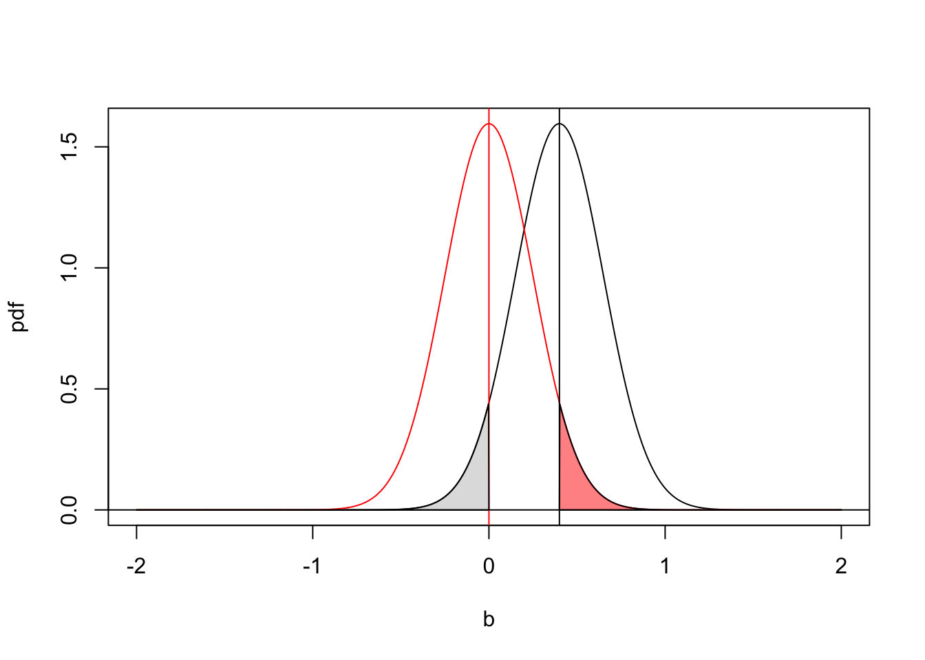
I will illustrate the relationship between confidence intervals and hypothesis test with an example below. Here I assume a parameter of interest was estimated to be 0.4 with a standard error of 0.25. The black line shows the probability density function for the population parameter given the observed data set. The grey shaded region corresponds to our confidence level that the true population parameter is less than zero. The red line shows the expected sampling distribution if the null hypothesis is true (\(b_1=0\)). The shaded red region is the probability of observing a parameter value greater than 0.4 if the null hypothesis is true. Because the width of the red and black distributions are equal (determined by the standard error of the parameter value) the area of these shaded regions are identical. For a two-tailed test with an alpha of 0.05, you would reject the null hypothesis if the area of the shaded region is less than 0.025 (divide 0.05 by to to account for both tails of the distribution).
4.7 False positives and negatives
The use of NHST takes as binary view of the world. First there is the truth: is the true population parameter 0 (null hypothesis) or not? Secondly, there is the conclusion from our study: We either reject null hypothesis or we fail to reject it. These give four possible outcomes:
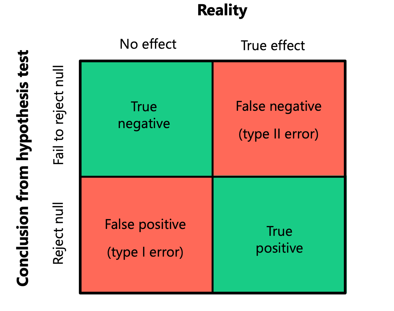
The good outcomes: There are true positives: you reject the null hypothesis and in reality the null hypothesis is not true There are true negatives, you fail to reject the null hypothesis and in reality the null hypothesis is true
The bad outcomes: False positive (type I error): you reject the null hypothesis when in reality the null hypothesis is true False negative (type II error): you fail to reject the null hypothesis when in reality the null hypothesis is not true
A useful analogy is with a covid test. You either have covid or you do not. If the test comes out positive when you don’t have covid this is a false positive and if the test comes out negative when you have covid this is a false negative.
We often want to know the probability that a given NHST is a false positive or false negative, however in practice it is impossible to know. What we can calculate, however, is the probability of a false positive or false negative conditioned on the null hypothesis either being true or false.
4.7.1 False positive rate when null hypothsis is true
If the null hypothesis is true (b = 0) then the probability of a false positive is equal to alpha. For example, if we reject the null hypothesis when p < 0.05, and we analyzed many datasets where the null hypothesis is true, we would reject the null 5% of time. These would be false positives because we would reject the null hypothesis even though the null hypothesis is true.
4.7.2 False negatives and power analyses
On the other hand, if there is a true effect, what is our probability of not rejecting the null hypothesis (a false negative)? This will depend on the magnitude of the true population parameter and then standard error, which will decrease with sample size. An intuitive way to think about this is that if the true parameter is small, we need small standard errors to differentiate that parameter from zero, and doing this requires larger sample sizes.
Another way of looking at this is, if the true population parameter does not equal zero, what is the probability I reject the null hypothesis in my study. This is often referred to as the statistical power of a test:
Power = 1 - P(false_negative)
To know the power of a specific test again need to know the true population parameter and the standard deviation of the errors. In practice you will rarely know these values. However, before you do an experiment, you can think about what the minimum effect size (e.g. magnitude of parameter value, which could be a difference between treatments or a regression slope) you would want to be able to detect. Generally, when you conduct an experiment or collect field data, you do it to test a hypothesis that one dependent variable is associated the value of another independent variable. Think about what the minimum effect size would be for your hypothesis to have practical importance. Then think about how noisy you expect the errors to be. This is often best done by looking for similar studies that measured the same dependent variable. Once you have a minimum effect size of interest, and an estimated standard deviation of the errors, you can calculate the power of your study under these conditions. In some cases there are formulas you can use to solve for the statisitcal power of a test, but a very general and easy way to calculate the power of your study is through simulation.
In this example, I want to conduct an experiment to measure the effect of ocean acidification on the growth rate of coral. I have one treatment with current pH levels and one with expected pH levels in the year 2100. My dependent variable is growth rate in % of body weight per day, and the minimum effect size that I think is biologically meaningful is -0.03%. Based on previous studies, I expect the standard deviation of the errors to be 0.05%. How many replicates per treatment would I need to have a 80% of detecting a the true effect?
To answer this question, I first need to write down an equation to generate the data of interest:
rep_N <- 10 #number of replicates per treatment
effect_size<- -0.03
sigma <- 0.05
pH<- c(rep(0,rep_N),rep(1,rep_N)) # generate dummy variable for pH (0 = current, 1 = future)
growth<- effect_size * pH + rnorm(rep_N*2,0,sigma)
plot(factor(pH),growth,xlab="pH",ylab="growth rate (%/day)")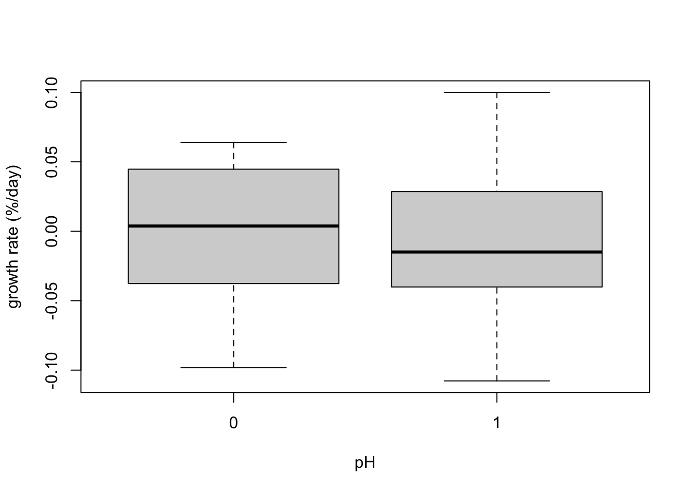 The variable ‘growth’ represents the simulated dependent variable, which depends on the treatment (pH level) and an error term. Notice that I didn’t add an intercept in this model, because it would not affect the power analysis. If you don’t believe this you can adapt the simulation to check. The code above generates one random data set, for which we can fit a linear model and check if we reject the null hypothesis for the difference in growth in current (0) and future (1) conditions. In this case:
mod<-lm(growth~pH)
summary(mod)
Call:
lm(formula = growth ~ pH)

Residuals:
      Min        1Q    Median        3Q       Max
-0.099456 -0.031315  0.000209  0.040760  0.111305

Coefficients:
             Estimate Std. Error t value Pr(>|t|)
(Intercept)  0.001174   0.018311   0.064    0.950
pH          -0.012472   0.025895  -0.482    0.636

Residual standard error: 0.0579 on 18 degrees of freedom
Multiple R-squared:  0.01272,   Adjusted R-squared:  -0.04213
F-statistic: 0.232 on 1 and 18 DF,  p-value: 0.6359
we see that in this simulated experiment, we would have failed to reject the null hypothesis, even though we know there was a true effect in the model used to generate the simulated data. However this is just one simulation, to get estimate the power of this test, we need to simulate many data sets and then calculate the fraction of times we reject the null. I can do this with a for loop:
rep_N <- 10
effect_size<- -0.03
sigma <- 0.05
p<-rep(NA,1000)
for (i in 1:1000){
pH<- c(rep(0,rep_N),rep(1,rep_N)) # generate dummy variable for pH
growth<- effect_size * pH + rnorm(rep_N*2,0,sigma)
mod<-lm(growth~pH)
p[i]<-summary(mod)$coefficient[2,4]
}

power = sum(p<0.05)/1000
power
[1] 0.225In the for loop I generated 1000 datasets, conducted a null hypothesis test with alpha of 0.05, and counted the fraction of datasets where I rejected the null. In this case, with the number of replicates set to 10 per treatment, we only rejected the null hypotheses in about 22% of the experiments, even though we know that there is a true effect. If you think about all the work it takes to conduct en experiment, you probably want to have better than a 25% of detecting an effect in the case that your hypothesis is actually true. This suggests for this study, we should probably use a higher sample size. We can estimate how big of a sample size we need by running the code above with different numbers of replicate per treatment (rep_N), with a nested for loop.
rep_N <- seq(2,100,4)
effect_size<- -0.03
sigma <- 0.05
p<-rep(NA,1000)
power<-rep(NA,length(rep_N))
for (j in 1:length(rep_N)){
for (i in 1:1000){
pH<- c(rep(0,rep_N[j]),rep(1,rep_N[j])) # generate dummy variable for pH
growth<- effect_size * pH + rnorm(rep_N[j]*2,0,sigma)
mod<-lm(growth~pH)
p[i]<-summary(mod)$coefficient[2,4]
}
power[j] <- sum(p<0.05)/1000
}
plot(rep_N,power)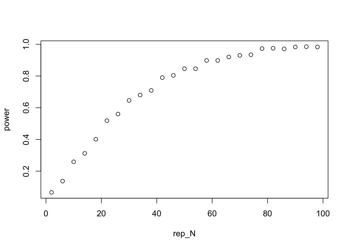 The plot above shows the probability of rejecting the null as a function of the number of replicates per treatment. We can see in this case, that to have a roughly 80% chance of rejecting the null we would over 40 replicates per group! It is always a good idea to run these types of simulations before you conduct your experiment and decide on sample sizes. You can adapt the code above to model and kind of experiment or field survey. If you are going to go through the trouble of running an experiment to test a hypothesis, you probably want to avoid failing to rejecting the null hypothesis in the case your hypothesis was actually right.
4.8 Multiple tests
Many times in scientific papers you see the authors conduct many hypothesis tests in one analysis. This could either be because they test whether many independent variables are associated with changes in a dependent variable, or they might look at how one independent variable affects many dependent variables. An example of the later case would be a paper that looks at how elevated temperatures affect zebrafish, and they measure many different dependent variables to quantify the effect of temperature. For example they could measure growth rates, different aspects of behavior, multiple stress hormones, ect.. The danger with this is that if you conduct enough hypothesis tests you will frequently find ‘statistically significant’ results, even if the null hypothesis is true.
Problem 4.3 For example, assuming the null hypothesis is true, the probability of rejecting the null with an alpha of 0.05, is 5%. Assuming the null hypothesis is true in each case, what is the probability of observing at least one ‘statistically significant’ result with an alpha of 0.05, when you conduct 10 null hypothesis significance tests?
It is easier to answer this question if we calculate the probability of not finding the significant result in any of the 10 tests, which is 1 - P(1 or more significant test). The probability of not finding a significant result in one test is 1- alpha, or in our case, 0.95. If we assume the null hypothesis is true, then the probability of not finding a significant result in one test should be independent of other tests. So to calculate the joint probability not finding a significant result in 10 tests, we just take the product of the individual probabilities:
alpha = 0.05
N_tests = 10
(1-alpha)^10
[1] 0.5987369Thus if we conduct 10 tests, the probability that at least one of them will be significant even though the null hypothesis is true is about 40%. This means you should be skeptical of studies that report many tests, and only 1 or 2 marginally significant results, because you would expect to see results like this even when the null hypothesis true. This means that the probability of a reporting a false positive result in a paper increases with the number of hypothesis tests conducted. An even worse practice is to conduct many test and then only report or focus on the select few that were significant.
One way researchers attempt to reduce the probability of reporting a false positive in a paper is to lower the threshold for declaring a result significant with the number of tests conducted. The simplest of these corrections is called the Bonferroni Correction which simply divides alpha by the number of hypothesis tests conducted in the analysis. So if I conducted 10 hypothesis tests, I would divide alpha by 10, and only reject the null when the p value for a test is less than alpha/10, or 0.005.
4.9 Common pitfals with the use of NHST
Below I outline some of the most problematic uses of NHST.
4.9.1 Statistical significance does mean biological or practical significance
Just because an independent variable is “statistically significant” does not mean that the variable has any practical importance for the problem at hand. For example, if a study estimates reports that a drug reduces blood pressure by 0.5 mmHg (about 0.5% of a typical value) with a standard error of 0.1, this result is statistically significant, but the effect is so small that it is probably not worth prescribing the drug. Standard errors are inversely proportional to the square root of sample size, thus if we have very large sample sizes, we can detect smaller and smaller “effect sizes”. With a large enough data set almost test will become significant, but this does not mean that the variable is practically important.
4.9.2 The null hypothesis is almost always false
This is closely related to another problem in that for most relevant biological questions the null hypothesis that the parameter of interest is exactly zero is almost certainly false. For example if we want to compare some variable of interest between two genotypes, or environments, or management policies the chance that there is exactly no difference between the groups, or a regression slope is exactly zero is probably very low. Thus whether or not we reject the null hypothesis is really just a matter of how much data we collect. This again emphasizes the need to pay attention to effect sizes and the practical significance of our parameter estimates.
4.9.3 Not staistically significant does not mean “no effect”
As shown in the section on false negatives, even when your hypothesis is true, you can fail to reject the null hypothesis. However it is very common for researcher to misinterpret ‘non-significant’ results to mean no effect. In fact, many studies are underpowered and don’t have sample sizes large enough to reliably reject the null hypothesis even when their alternative hypothesis is true.
4.9.4 p-values do not tell you the probability your hypothesis is true
A p value tells you the probability of observing your data/parameter conditional on the null hypothesis being true. 1-p does not, however, represent the probability your hypothesis is true. For example, consider a case where we know that only one gene out of 10,000 genes in a genome controls a specific developmental disorder, but we don’t know which gene it is. If we did a screening test for each gene, and then used NHST, we would expect about 500 cases where we reject the null hypothesis at an alpha of 0.05. Yet we know that the hypothesis that a specific gene controls the developmental order is only true for 1 out all of the tests. Thus the our hypothesis is true only for one out of 500 significant tests.
4.9.5 Arbitrary cutoffs
One of my least favorite aspects of statistical significance is that results with p-values less then 0.05 tend to be treated as unambiguous established facts and results with p-values > 0.05 are no true effect. However nothing magical happens as p-values go from 0.0501 to 0.0499. These values are essentially identical, so it seems absurd to come to completely different conclusions for the two cases.
4.10 My advice
The two most important pieces of information you get when you fit a linear model are the values of the parameter estimate and their standard errors. From these two pieces of information you can very closely estimate 95% CI, which also will tell you the result of a NHST that the parameter = 0. In my opinion, p-values and NHST are entirely optional, while effect sizes and standard errors/CI are mandatory when reporting scientific results. Never just say, oh this variable is statistically significant, and nothing else. Remember it is the actual value of the estimated parameter that tells you the practical importance of your finding, and the standard error of a parameter value tells you the uncertainty of that estimate. Always be skeptical if you read in a paper or in the news that a variable is statistically significant when they don’t report the effect size. Finally, try to avoid binary decisions. I think it is probably human nature to want to come to unambitious decisions in the face of uncertainty, and in science we also want our conclusions to be reached in an objective way. This helps explain the popularity of NHST in that it provides a way to come to binary conclusions in a way that is perceived as objective. However just because it is conventional practice to declare results with p< 0.05 “statistically significant and p > 0.05 not significant, does not change the fact that p = 0.0499 is effectively identical to p = 0.0501 and it is absurd to come to completely different conclusions for these two cases. It is better to think on a continuous scale of evidence against the null hypothesis.Finally, before you do a study, run simulations with plausible values for parameters and errors. See how large your sample sizes need to be to detect meaningful effects.
4.11 What you should know
1. What is a p-value? How to interpret p-values reported in the lm() output
2. You should be able to conduct a power analysis by simulation
3. You should know the relationship between 95% CI and NHST with an alpha of 0.05
4. You should know that it is never OK just to say “variable X was statistically significant” and not report the effect size and standard error or confidence intervals.
5. You should be aware of how the probability of one or more false positives increases with the number of tests