2 Fitting models to data
2.1 Recap
In chapter 1 we introduced the general structure of a linear model. We will use linear models for the entire class to describe and communicate patterns in data, estimate how certain we are about the estimated relationships among variables, tests hypotheses, and make predictions.
The first step of our analysis begins with deciding which variable we want to model (what is the dependent or response variable), and what independent variables we think the dependent variable depends on. Typically this is something you should decide before you start your study whether you are doing an experiment or collecting observational data. For example, if we were interested in the effect of nitrogen on plant growth we might conduct an experiment where we measure the growth rate of plants at different soil N levels. In this case, it is clear that the variable we are interested in modeling is plant growth, and we want to model it as a function of N:
\[growth = f(N)\] The \(f(N)\) means that plant growth is a function of N. In theory, we could use any equation or function but in this class we will focus on general linear models
Problem 2.1: Write down a linear model to predict plant growth as a function of N. Describe each parameter in the model:
Answer:
\(\mathbf {\hat y} = b_0 + b_1 \mathbf {N}\)
\(b_0\): expected plant growth when N = 0
\(b_1\): the expected increase in plant growth per unit increase in N
2.2 Fitting models to data
After we have specified the model, the next step is to fit the model to the data. This means finding the parameter values that make the model most accurately match the data. We saw in chapter 1, that for simple models, you can get a rough estimate of parameters just by looking at a plot of the data. But ideally, we want a more precise and systematic way of fitting models to data. This is even more important for complex models with multiple variables for which visualizing all the relationships among variables on a 2-dimensional computer screen is difficult.
To fit a model to data we first need to quantitatively define what it means for a model to match data. In other words, we need to put a number on how well a model fits data. Once we have a quantitative metric for model fit, the next step is to search for the parameter values that optimize this metric.
An intuitive way of thinking about how well a model fits data is how closely the predictions of the model match the observations. The difference between observation and predictions are called errors residuals. Models that fit the data well should have small errors. It is straightforward to calculate the error for each observation, but then the question is how to we aggregate the errors for all of our data to come up with one number that quantifies how well our model matches the data.
The most intuitive thing to do would be to calculate the error for each observation and sum them. For example let’s consider a data set with just 3 observations \(\mathbf { y} = [4,5, 6]\). Here we have no independent variable, so we just want to find the parameter \(b_0\) that best fits the data:
\[\mathbf {\hat y} = b_0\]
If you wanted to pick a value for \(b_0\) to closely match the data, 5 would be a good choice:
| Observation | Prediction | Residual |
|---|---|---|
| 4 | 5 | -1 |
| 5 | 5 | 0 |
| 6 | 5 | 1 |
| sum | 0 |
We can see that for the first and 3rd observation, the model is off by 1. However, one residual is positive and one is negative so the sum of all the residuals is 0. Thus using the sum of all the residuals as a metric of goodness of fit has a problem in that even though our model doesn’t fit the data perfectly, the sum of the errors equals zero. This is particularly problematic if we want to compare how well models fit different data sets. For example, if we had a second data set \(\mathbf { y} = [0,5, 10]\), with \(b_0 = 5\), the sum of the residuals again equals 0, in spite of the fact that the typical distance between observation and prediction is much higher:
| Observation | Prediction | Residual |
|---|---|---|
| 0 | 5 | -5 |
| 5 | 5 | 0 |
| 10 | 5 | 5 |
| sum | 0 |
One way around this problem is to simply square the residuals and then sum them. If we do this for both example data sets we get the following:
| Observation | Prediction | Residual | Residual\(^2\) |
|---|---|---|---|
| 0 | 5 | -1 | 1 |
| 5 | 5 | 0 | 0 |
| 10 | 5 | 1 | 1 |
| sum | 0 | 2 |
| Observation | Prediction | Residual | Residual\(^2\) |
|---|---|---|---|
| 0 | 5 | -5 | 25 |
| 5 | 5 | 0 | 0 |
| 10 | 5 | 5 | 25 |
| sum | 0 | 50 |
We see that the sum of the squared residuals, or \(SS_{Error}\) is lower for the first dataset, which is consistent with the fact that the predictions of the model are more accurate for the first dataset.
Problem 2.2: In the example above, we squared the residuals so that they don’t cancel each other out when we sum across observations. But couldn’t we have done other transformations to avoid this problem? Think of two other ways of quantifying errors to avoid negative and positive residuals don’t cancel each other out.
One simple way to keep positive and negative residuals from canceling each other out would be to sum the absolute value of the residuals. Alternatively we could raise the residuals to the 4th power. These different ways of counting errors have consequences for how influential specific observations are. For example we when square errors, large errors have a disproportionate influence on the goodness of fit compared to smaller errors, while if we just used the absolute value of residuals all residuals contribute to the total in proportion to their size.
So there are many criteria we could use to quantify the goodness of fit, but in practice, when our dependent variable is continuous and we assume that errors are normally distributed, we typically use the \(SS_{Error}\). The method of fitting statistical models to data by finding the parameters that minimize \(SS_{Error}\) is often referred to as Ordinary Least Squares or OLS. To understand why we primarily use Ordinary Least Squares and not, for example, Ordinary Least Absolute Values, we need to understand a little bit about probability and likelihoods.
2.3 Discrete probability distributions
A deeper and more fundamental goal of fitting models to data, is to find the parameters of the model that make the data most likely. To be able to understand this we need to review some basics about probability.
Probability is easiest to think about when we have a discrete number of outcomes. For example, in a coin flip there are two outcomes: heads or tails. If the coin is a fair coin, each outcome has equal probability:
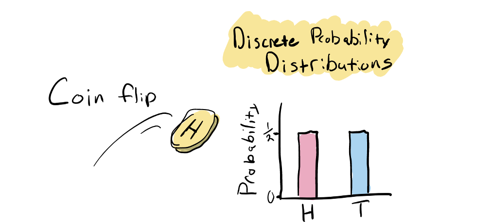
A probability distribution is simply a function that describes the probability of all possible outcomes. In the case of a fair coin there are just two outcomes, each with a probability of 0.5. An important point about all probability distribution functions is that the sum of the probabilities for all possible outcomes equals one (e.g. 0.5 (probability of heads) + 0.5 (tails) = 1). Other examples of a discrete probability distributions would be the probabilities of throwing rock, papers, or scissors in a game of rock-paper-scissor shoot, or the probabilities of rolling 1-6 on a 6-sided dice.
2.4 Probability density functions
The examples above are discrete probability distributions because there are a finite set of outcomes the observations can take. For continuous data, such as height, weight, temperature, etc., there are, in theory, an infinite number of values these measurements can take. For example, someone’s height could be 170.1 cm, or 170.01 or 17.00000001 cm (although in practice we generally only measure down to some level of precision). As a result the probability of observing exactly any specific value is zero!
For continuous variables, it doesn’t make sense to talk about probabilities of specific outcomes because the probability of any outcome is zero. Instead, for continuous variables we use probability densities. A probability density function is a function that defines the probability density for a particular value of a random variable. A very important probability density function for this course is the normal distribution (AKA Gaussian distribution), which is defined by its mean and standard deviation, and looks like the following:
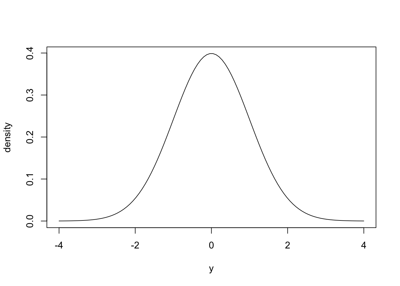
The plot above shows a probability density function of a normal distribution with mean = 0 and standard deviation = 1. The probability density for \(y\) is shown on the \(y\)-axis. Intuitively, you can look at this plot and see the probability density is highest around the mean (0) and decreases for higher or lower values. You can think of probability densities as the relative likelihood of observing specific values. In the example above, the probability density at \(y = 0\) is roughly 0.4, and at 1 is roughly 0.2, thus values of \(y\) very close to 0 are twice as likely to be observed as values very close to 1.
More formally, the probability density is defined as the probability of observing a value of \(x\) between \(x\) and \(x+\Delta\) as \(\Delta\) approaches zero. While the absolute probability of observing any specific value of a continuous variable is zero, the relative likelihood of observing values close to a specific value are proportional to their probability density. Importantly, the integral of a probability density function equals 1, and the probability of observing a value of \(x\) within a specific range (e.g. between 1 and 2) is equal to the area under the curve in this interval. This will be important later in the course.
The equation that gives the probability density for the normal distribution is:
\[ f(x)= \dfrac{1} {\sigma \sqrt{2 \pi}} e^{-\dfrac{1}{2}\left(\dfrac{x-\mu}{\sigma}\right)^2} \]
For now I just want you to note the parameters in the equation \(\mu\), the mean or predicted value of \(x\), and the standard deviation, \(\sigma\). Also notice that squared errors \((x-\mu)^2\) already show up in the normal probability density function, which already gives a clue about why we work with squared residuals in OLS. You can think of \(\mu\) as determining where the distribution is centered, and \(\sigma\) determining the width of the distribution (when sigma is large the distribution is wide). If these parameters \(\mu\) and \(\sigma\) are known, then we can calculate the probability density for an observation, \(y\). In R you can calculate the density function of the normal distribution using the dnorm() function (the “d” stands for density, and “norm” for normal distribution). The syntax of the function is:
dnorm(y, mean = 0, sd = 1)Importantly, we can use this probability density function to calculate the relative likelihood of a particular observation. Where \(y\), is an observation and the mean = \(\hat y\) or the predicted value for that data point, and sd is the standard deviation, \(\sigma\), of the normal distribution.
Problem 2.3 A statistical model predicts \(\hat y =5\), with a \(\sigma =2\), but the observed value of \(y\) was 6.2. What is the probability density of this observation given the model?
We can answer this question using the dnorm function
obs = 6.2
pred = 5
sigma = 2
pd =dnorm(obs,pred,sigma)
pd
[1] 0.1666123We can inspect this answer visually, by plotting out the normal probability density function for \(\mu = 5\), \(\sigma = 2\) for a range of values and then plotting out the pd for \(y = 6.2\) (red point):
y<-seq(0,10,length.out=100) #range of x values
pred = 5
sigma = 2
pdf =dnorm(y,pred,sigma)
plot(y,pdf,'l')
abline(v=5)
text(6, .03, "predicted y")
text(7.5, pd, "observed y",col='red')
points(6.2,pd,col='red')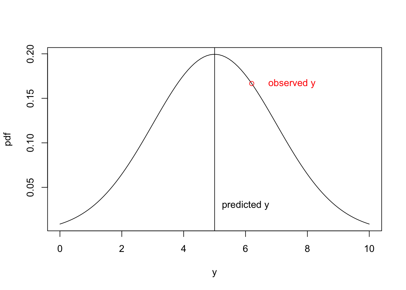
In the example above, we only have one data point. If we wanted to find the parameters that maximized the likelihood of this data point, where the model is: \[\hat y = b_0\] then it is clear that \(b_0\) should equal the value of the data point: \(y\). However in real applications, we have more than one observation. The question then is how do we maximize the likelihood of the data when there are multiple observations? To answer this question, we need to understand joint probabilities.
2.5 Joint probability
Problem 2.4 If you roll a 6-sided dice two times, what is the probability of rolling two 6’s?
The probability of two independent events occurring is equal to the product of their individual probabilities. The probability of rolling a 6 is 1/6 and thus the probability of rolling two sixes is 1/6 * 1/6 = 1/36.
The key point in the example above is that when observations are independent their joint probability is the product of probabilities of each observation. Thus if the errors are independent, the likelihood of a dataset given a particular set of parameters is equal to the product of the probability density function for each observation. As mentioned in Chapter 1, independent errors is an important assumption of general linear models, and here we can partially see why: our calculation of the likelihood of the data given a parameter set assumes each error is independent.
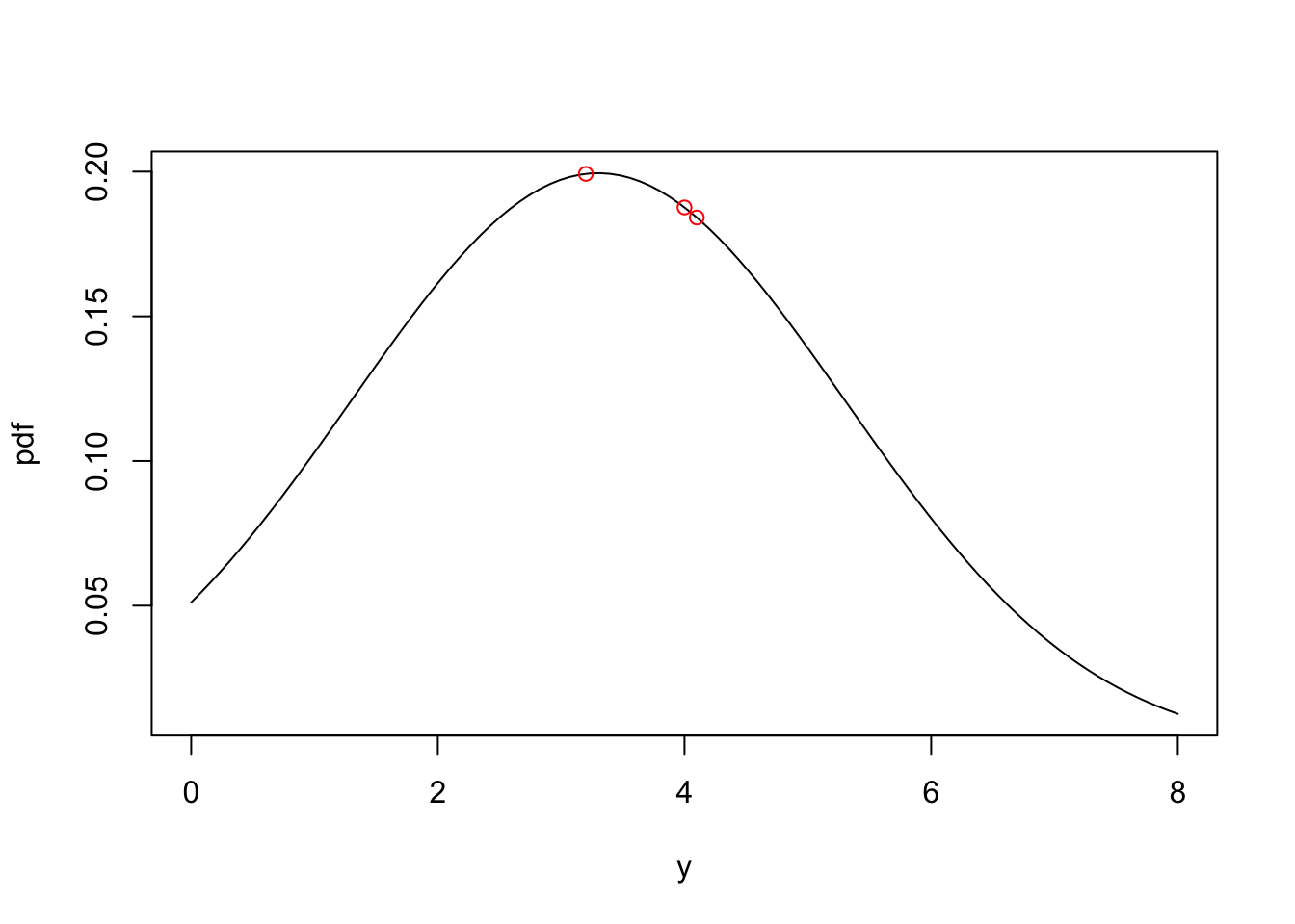
Problem 2.5 What is the likelihood of observing the dataset \(\mathbf{y}\) = [3.2, 4.1, 4.0] assuming y is a normally distributed random variable with mean = 3.3 and \(\sigma\) = 2?
We can calculate the likelihood of the data set given the model parameters by taking the product of the probability density for each observation:
b0=3.3
sigma=2
dnorm(3.2,b0,sigma) * dnorm(4.1,b0,sigma) * dnorm(4.0,b0,sigma)
[1] 0.006882611We can visualize this by looking at the probability density function (often shortened to pdf) for the parameters \(b_0=3.3\) and \(\sigma=2\). Each of the red points corresponds to the probability density for the 3 observations, and the likelihood of the data given the parameters is given by the product of the tree probability densities.
2.6 Maximum Likelihood Estimation
Problem 2.6 Can you find a value of \(b_0\) that makes the observed data more likely? What is the value of \(b_0\) that maximizes the likelihood of the data?
One way to answer this question is by brute force: we just try out a range of values for \(b_0\) and see which one results in the highest likelihood. We can do this with a for loop.
# Create vector of length 100 with b0 values between 2 and 6
b0=seq(2,6,length.out=100)
# Create vector of equal length with NA values (NA = Not Available / Missing Value)
likelihood = NA * b0
sigma=2
for (i in 1:length(b0)){
likelihood[i] = dnorm(3.2,b0[i],sigma) * dnorm(4.1,b0[i],sigma) * dnorm(4.0,b0[i],sigma)
}
plot(b0,likelihood,'l')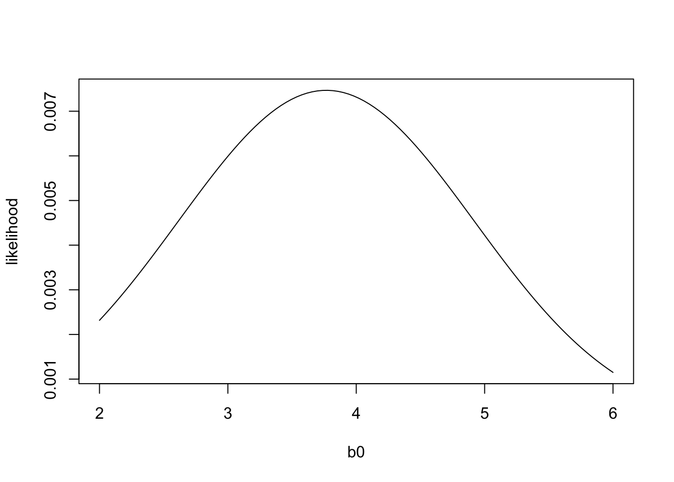 The plot above shows the likelihood of the data for different values of \(b_0\). The value of \(b_0\) that maximizes the likelihood of the data is called the Maximum Likelihood Estimate. We can see that the likelihood of the data is maximized when \(b_0\) is less than, but close to 4. Your intuition would probably tell you that the value of \(b_0\) that best matches the data would be equal to the mean of \(y\). And if we compare the mean of \(y\) to the likelihood function, we see in fact the maximum likelihood estimate of \(b_0\) is the mean of \(y\):
plot(b0,likelihood,'l')
abline(v = mean(c(3.2,4.1,4.0)), col="red", lwd=3, lty=2)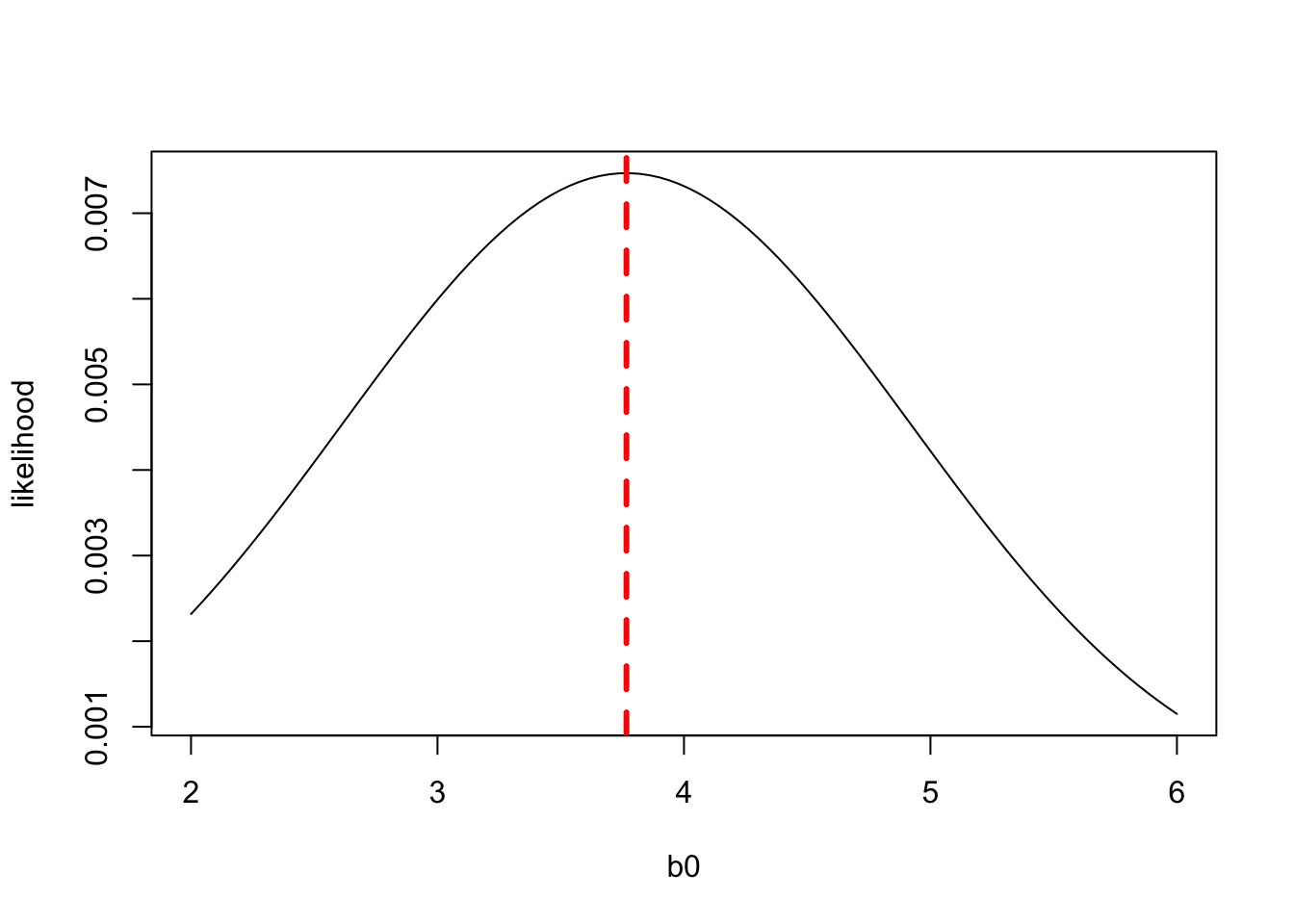
Problem 2.7 So far we have assumed \(\sigma = 2\), but in general, \(\sigma\) isn’t known, and has to be estimated from the data. Given that \(b_0\) = mean(\(y\)), what is the value of sigma that maximizes the likelihood of the data?
We can again use brute force to estimate sigma, with \(b_0\) set to the mean of \(y\).
b0=mean(c(3.2,4.1,4.0))
sigma=seq(0.1,4,length.out=400)
likelihood = NA * sigma # in
for (i in 1:length(sigma)){
likelihood[i] =  dnorm(3.2,b0,sigma[i]) * dnorm(4.1,b0,sigma[i]) * dnorm(4.0,b0,sigma[i])
}
plot(sigma,likelihood,'l')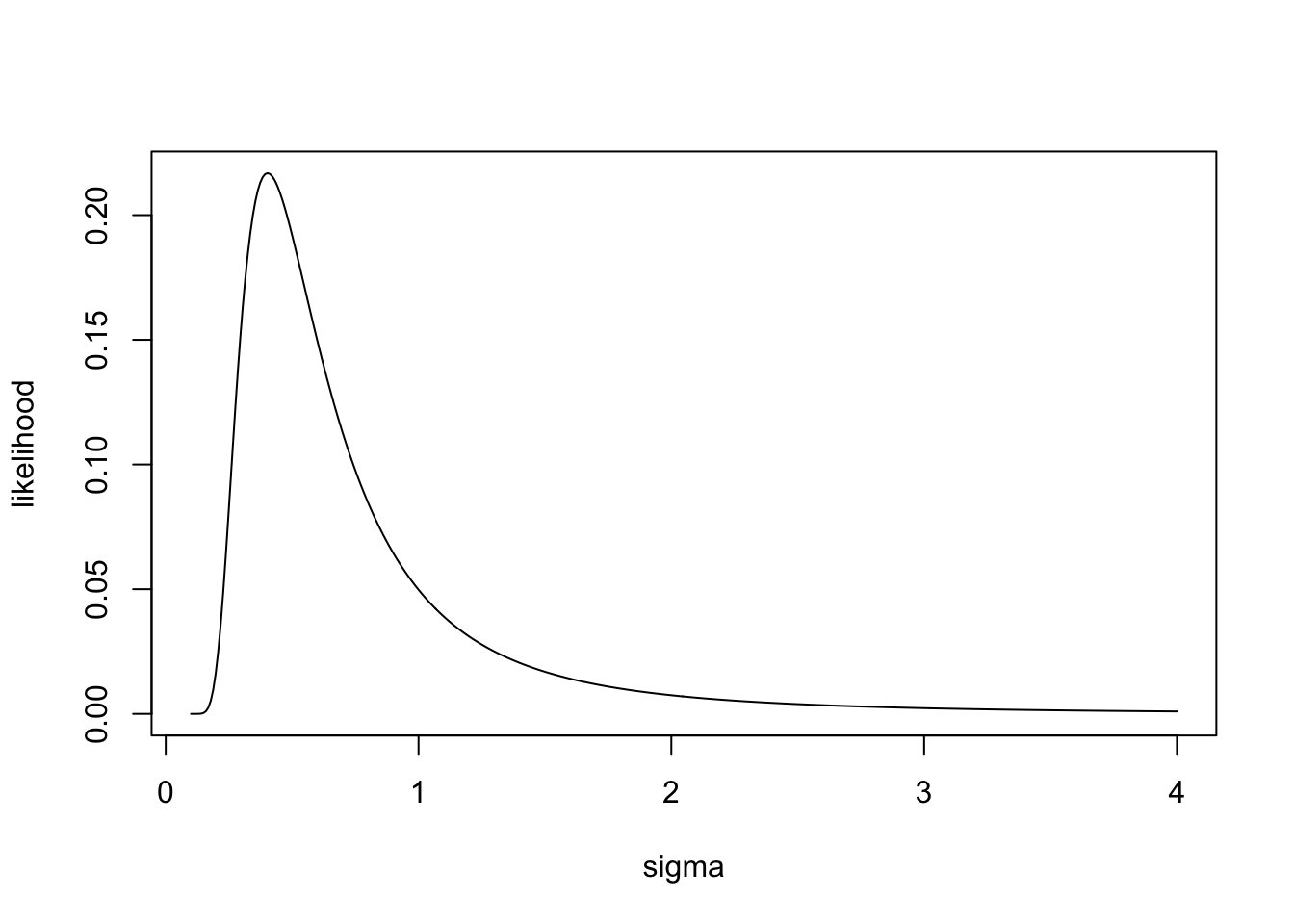
sigma[which.max(likelihood)][1] 0.4030075We see that the likelihood of the data is maximized at an intermediate value of \(\sigma\). If \(\sigma\) is too small the pdf is very narrow, and observations far from the mean are very unlikely, but if \(\sigma\) is too wide, then the pdf gets spread across a wide range of possible values, and the overall likelihood is low. It turns out that the \(\sigma\) that maximizes the likelihood is equal to the square root of the sample variance,\(s\):
\[s^2 = \dfrac{\sum_{n=i}^{n} (y_i-\hat y_i)}{n} \] where \(n\) is the number of data points.
The estimate of \(\sigma\) that maximizes the likelihood of the data is just the square root of the the sample variance, \(s\). Thus, \(s\) is the maximum likelihood estimate of the true population \(\sigma\).
However you may notice that, you get a slightly different answer if you just calculate the standard deviation of the data, in R using the function sd(). This is because the maximum likelihood estimate of \(\sigma\) is slightly biased. It will on average underestimate the true population standard deviation. This is because if there is one parameter in the model and 3 data points, there are only 2 degrees of freedom to estimate the standard deviation. For example if we had only one data point, the mean would equal the value of the one data point, and the estimate of the variance would equal zero, when in fact we don’t have enough information to estimate variance from a single data point. Thus the unbiased estimate of the population variance is:
\[s^2 = \dfrac{\sum_{n=i}^{n} (y_i-\hat y_i)}{n-1} \]
However for large datasets (large \(n\)) you basically get the same answer.
The important take-home message here is that by taking the product of the probability densities for all observations from the probability density function we can calculate the likelihood of the data for a given parameter set. When we fit our model to data, the goal is to find the parameter set that maximizes the likelihood of observing the data.
The parameter set that maximizes the likelihood function is called the maximum likelihood estimate.
2.6.1 Ordinary Least Squares and Maximum Likelihood give the same answers when errors are normally distributed
Below I will show that if errors are normally distributed then the parameters that maximize the likelihood function are the same parameters that minimize the sum of squared errors. So again, the likelihood of observing a dataset, given a model with parameters \(\theta\) is calculated by taking the produce of the probability densities of the individual observations:
\[ L(y|\theta)= \dfrac{1} {\sigma \sqrt{2 \pi}} e^{-\dfrac{1}{2}\left(\dfrac{y_1-\hat y_1}{\sigma}\right)^2} \times ... \times \dfrac{1} {\sigma \sqrt{2 \pi}}e^{-\dfrac{1}{2}\left(\dfrac{y_n-\hat y_n}{\sigma}\right)^2} \]
You might have already noticed a difference between ordinary least squares and maximum likelihood. In OLS we add the squared errors together, but in MLE we multiply the probability densities. However, if we take the log of the likelihood function, it turns multiplications into additions:
\[ \log{L}= \log\left({\dfrac{1} {\sigma \sqrt{2 \pi}}}\right){-\dfrac{1}{2}\left(\dfrac{y_i-\hat y_i}{\sigma}\right)^2} + ...+ \log\left({\dfrac{1} {\sigma \sqrt{2 \pi}}}\right){-\dfrac{1}{2}\left(\dfrac{y_n-\hat y_n}{\sigma}\right)^2} \]
Since \(\sigma\) is the same for each term, we can factor out everything that doesn’t include a \(y\) or \(\hat y\).
\[ \log{L} = \log\left({\dfrac{n} {\sigma \sqrt{2 \pi}}}\right)-\dfrac{1}{2 \sigma^2} \left( \left( y_1-\hat y_1\right)^2 + ... + \left(y_n-\hat y_n \right)^2 \right) \]
which is the same as:
\[ \log{L} = \log\left({\dfrac{n} {\sigma \sqrt{2 \pi}}}\right)-\dfrac{1}{2 \sigma^2} \sum^n_{i=1} \left(y_i - \hat y_i\right)^2 \] While this still looks complicated, keep in mind that we don’t actually care what the absolute value of the log likelihood is, we just need to know the parameters that minimize the likelihood, and we can use the log likelihood because the parameters that maximize the log-likelihood also maximize the likelihood. By grouping terms that don’t depend on the linear model parameter (the \(b\)’s) in a linear model, we can simplify the equation to:
\[ \log{L} = C_1 - C_2 \sum^n_{i=1} (y_i - \hat y_i)^2 \] which is just
\[ \log{L} = C_1 - C_2 \times SS_{Error} \] Here we can see that the the log likelihood (and thus the likelihood) will be maximized when the \(SS_{Error}\) is minimized.
2.6.2 Take-home messages about the relationship between OLS and MLE
This is a rather long demonstration of how OLS is related to MLE for data with normal distributions. I don’t expect that you memorize these formulas, what is import though is that:
1. You have some idea of why we focus on the sum of squared errors as a measure of goodness of fit. We use \(SS_{Error}\) because it is fundamentally related to likelihood when errors are normally distributed.
2. You understand probability density functions because we will use them throughout the class.
3. After this course you might work on data sets where the dependent variable is not normally distributed. For example, if you work with binary data (e.g. presence/absence), or count data (values only take positive integer values), the errors will have a different error distribution. Maximum likelihood estimation is a general technique for fitting models to data and can be used for any type of data. In this case, you will want to use Generalized Linear Models, which are different from the topic of this course (general linear models) in that they generalize to different error distributions (e.g. binomial, multinomial, poisson).
2.7 Optimization (how do we find the best parameters)
We have shown that you can estimate parameters by brute force (trying a wide rang of values) for each parameter in the model. However this becomes much more difficult when there are many parameters. The beauty of linear models, and a major reason why we use them so often, is that it is very easy to fit them to data. Because the predicted value of a linear model is a linear combination of the independent variables, where the effect of each independent variables is weighted by its parameter value, you can use linear algebra and calculus to solve for the parameter values that minimize the sum of squared errors. All statistical software packages use these calculations to estimate model parameters. In our class we will us the lm() function in R, which will return the optimal parameter values for the specified model.
The details of how one can analytically solve for the best parameters is beyond the scope of this class, but for those interested feel free to check out these resources on linear optimization (you probably need some experience with linear algebra to follow):
2.7.1 Non-linear optimization
In cases where the model is non-linear there is no analytical way to solve for the best parameters. In practice this means that that finding the best parameters is essentially done by trial and error. When there are many parameters, the brute force method is no longer feasible. Instead you generally provide a starting guess for the parameters, from which the \(SS_{Error}\) or log-likelihood can be calculated. Then various algorithms are used to search for parameters that can improve the fit. Non-linear models are beyond the scope of this class, but for an interesting introduction to non-linear optimization in the context of machine learning check out this video:
https://www.youtube.com/watch?v=IHZwWFHWa-w&t=421s&ab_channel=3Blue1Brown
2.8 Other important metrics of goodness of fit
As discussed above, we use \(SS_{Error}\) as a metric of the goodness of fit and optimize our models by finding the parameters that minimize \(SS_{Error}\). But \(SS_{Error}\) isn’t always the most useful metric for communicating how well our model fits the data. For example, we might want to know how far off the predictions of our model are on average, or we might also what to know how much of the variability in the data is explained by the independent variables in our model. In this section, we briefly discuss two additional but important metrics of goodness of fit: residual standard error and \(R^2\).
2.8.1 Residual standard error
The residual standard error (RSE) is defined as:
\[ \text{RSE} = \sqrt{\dfrac {SS_{Error}}{df}} \]
where \(df\) are the degrees of freedom, which is given by \(n - k\), where \(n\) is the number of data points and \(k\) is the number of parameters in the model. The residual standard error is also an unbiased estimate of the standard deviation of the errors, \(\sigma\).
To calculate the RSE you take the square root of the sum of the squared errors (\(\sum(y_i- \hat y _i)^2\)) divided by the degrees of freedom. You divide by degrees of freedom rather than the number of data points because if you have a model with \(n\) data points and \(n\) parameters, the model can fit the data perfectly. For example, with two data points, a regression line can go perfectly through the data, so we need more than 2 data points to be able to quantify the typical variability in the data.
The residual standard error essentially tells how close model predictions are to data on average. If a weather model predicts tomorrow’s temperature will be 20\(^{\circ}\)C but has a residual standard error of 5\(^{\circ}\)C, you should be prepared to encounter a wide range of conditions as shown in the following graph:
temp<-seq(0,40,length.out=100)
density <- dnorm(temp,20,5)
plot(temp,density,'l')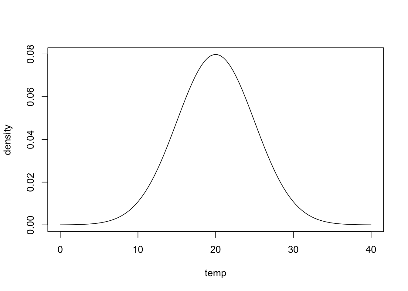
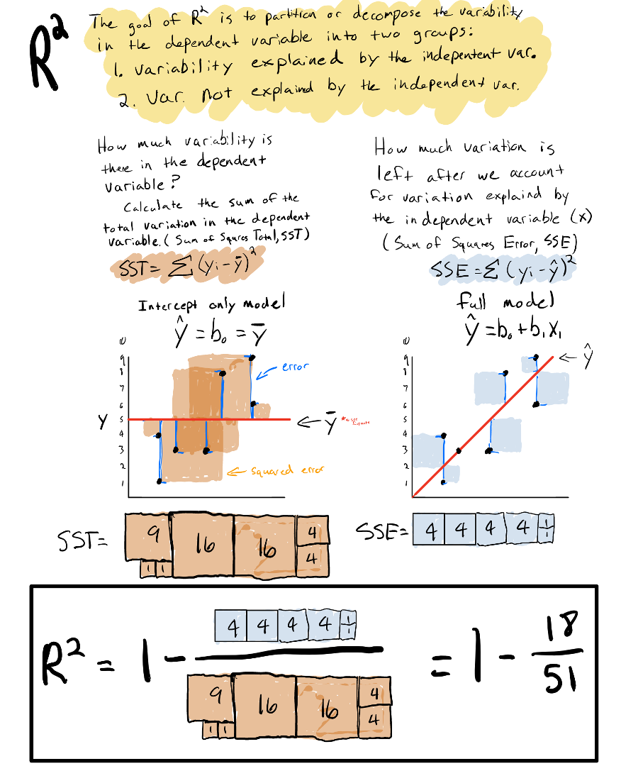
2.8.2 R-squared
Another useful way of quantifying goodness of fit is asking, how much of the variability in the data can be explained by the independent variables in the statistical model.
To do this, we can first quantify how much variability is in the data in the first place, by calculating the sum of squared errors in a model with no independent variables:
\[y=b_0\]
Where \(b_0\) is just the mean of the data.
Doing this is essentially the same thing as calculating the summed variance of the data. We call this the total sum of squares \(SS_{Total}\):
\[SS_{Total}=\sum(y_i- \bar y)^2\] where \(\bar y\) is the mean of the dependent variable.
The idea of \(R^2\) is to partition \(SS_{Total}\) into variation explained by the independent variables in the model \(SS_{Model}\) and variation not explained by the independent variables \(SS_{Error}\).
\[SS_{Total} =SS_{Model} +SS_{Error}\]
We already know how to calculate \(SS_{Total}\) and \(SS_{Error}\), and we can therefore calculate \(SS_{Model}\) as:
\[ SS_{Model} = SS_{Total} - SS_{Error} \]
We can then calculate what fraction of \(SS_{Total}\) is explained by the model by dividing both sides of the equation by \(SS_{Total}\):
\[ R^2 =\dfrac{SS_{Model}}{SS_{Total}} =\dfrac{SS_{Total}}{SS_{Total}} - \dfrac{SS_{Error}}{SS_{Total}} \]
which reduces to:
\[ R^2 =1 - \dfrac{SS_{Error}}{SS_{Total}} \]
\(R^2\) is a measure of the proportion of the variation in the dependent variable explained by the independent variables in the model. Because \(R^2\) is a proportion, its value will fall between 0 and 1. When it is 0, it means the model doesn’t explain any variability in the data, and when it is 1 it means that it explains all the variability in the data. For real data sets, \(R^2\) will fall in between 0 and 1. The closer the value is to 1, the more variation is explained by the model.
Below is an graphical and numerical demonstration of \(R^2\):
2.9 Introduction to transformations
Transformations involve converting a variable from one scale to another. Such transformations are sometimes useful to allow us to use general linear models (that assume linearity, normality and constant variance) to model data that don’t meet initially these assumptions. For example, cosider the data below that show the concentration of a drug in the blood of patients as a function of time (days) since the drug was taken, and the linear statistical model that was fit to the data:
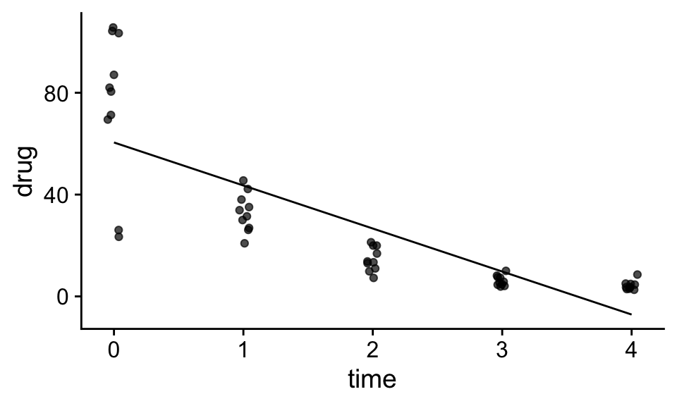
Question: Can you identify some problems with using the linear model above to model the data?
Probably the most striking problem with the above model is that the assumption that the concentration of the drug decreases as a constant rate per unit time is clearly not supported by the data. For example, going from day 0 to day 1 results in a drop of about 30 mg, while from day 3 to day 4, the drop is only around 5 mg. Instead we see that the rate of drop seems to depend on amount of the drug in the blood; when the concentration is high the drop is high. We also can see the the variance among the data points seems to systematically decrease with time as the concentration of the drug is lower.
Question: Can you think of a equation that might better represent the relationship between time and drug concentration?
The data in the example above, look like an example of exponential decay, were during each interval of time, some fraction In cases, when the growth or decay rate of a quantity is proportional the value of the quantity, we expect concentration to either exponential increase or decrease over time:
\[\hat y(t) = C_0 e^{rt}\] Here, C_0 and r are the parameters of the model, representing the intial concentration, and growth rate respectively, and in terms of a statistical model, t, or time is the dependent variable. We can tell this model is not linear in the parameters because the parameter r shows up in the exponential along with the independent variable t.
However if we log transform borth size of the equation:
\[\ln y(t) = \ln(C_0) + r t\] We see that this has the same structure of a linear model
\[\ln \hat y = b_0 + b_1 t\] where,
\[b_0 = ln(C_0)\] \[b_1 = r\] Thus if our data were generated by an exponential process, either exponential growth or decay, than log transforming the dependent variable allows us to fit a linear statistical model:
mod<-lm(log(drug)~time,df)
df$pred<-predict(mod)
ggplot(df,aes(x=time,y=log(drug)))+
  geom_jitter(width=.05,height=0,alpha=.7)+
  geom_line(aes(x=time,y=pred))+
  theme_cowplot()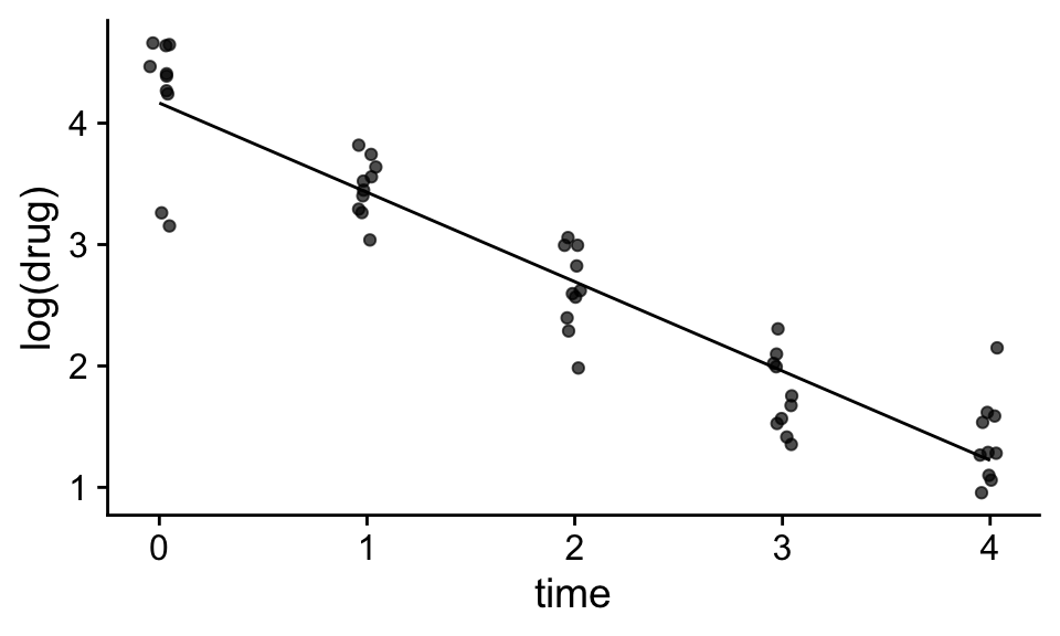
We can from the plot above that converting the dependent to log scale allows us to us a linear model to a non-linear relationship. We can also see that transforming the dependent variable solved the issue of non-constant variance as well. In linear scale, the variability appears to be proportional to the average of the dependent variable, however in log scale, the variability appears to be more or less constant across the data set.
This brings up a general point, if we transform the dependent variable, it will not only affect the relationship between the dependent variable and the independent variables, it will also change the distribution of the error terms. In the example above, transforming the dependent variable solved both the linearity and constant variance, but this will not always be the case.
2.9.1 Converting back to linear scale
While transforming variables can sometimes make it easier to fit statistical models to data, the are often easier to interpret in their original scale. Thus we will often want to convert prediction of our model back to the original scale, or convert the parameters of our linear statistical model back to the parameters of the original non-linear equation.
We can convert the predictions of our model from the transformed to originla scale by applying the inverse function of our transformation. Because exponentiation undoes taking the log transformation, if we apply the exponential function to our prediction, we can convert predictions back to linear scale:
mod<-lm(log(drug)~time,df)
df$ln_pred<-predict(mod)
df$pred<-exp(df$ln_pred)
ggplot(df,aes(x=time,y=drug))+
  geom_jitter(width=.05,height=0,alpha=.7)+
  geom_line(aes(x=time,y=pred))+
  theme_cowplot()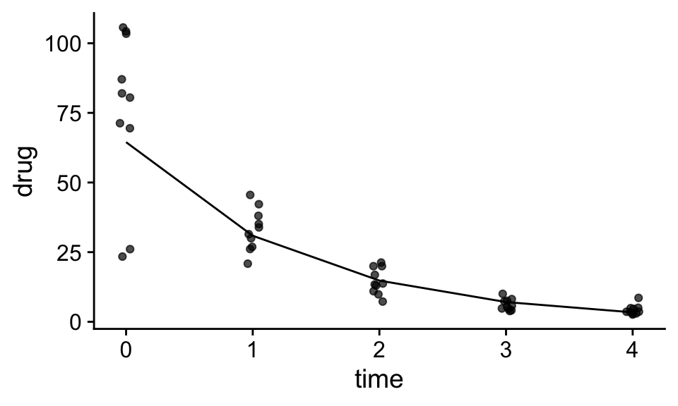
To relate the linear statistical model parameters back to the parameters of the orininal non-linear equation, we simply need to look at the mathematical relationship between the two. This will depend on the non-linear equation and transformations applied, but in our case, because \(b_0 = \ln(C_0)\), and \(b_1 = r\), we know that \(C_0 = e^{b_0}\) and \(r = b_1\).
Thus by looking at the estimated linear parameters:
mod<-lm(log(drug)~time,df)
summary(mod)
Call:
lm(formula = log(drug) ~ time, data = df)

Residuals:
     Min       1Q   Median       3Q      Max
-1.01302 -0.19548  0.06071  0.29972  0.92671

Coefficients:
            Estimate Std. Error t value Pr(>|t|)
(Intercept)  4.16630    0.09376   44.44   <2e-16 ***
time        -0.73597    0.03828  -19.23   <2e-16 ***
---
Signif. codes:  0 '***' 0.001 '**' 0.01 '*' 0.05 '.' 0.1 ' ' 1

Residual standard error: 0.3828 on 48 degrees of freedom
Multiple R-squared:  0.8851,    Adjusted R-squared:  0.8827
F-statistic: 369.7 on 1 and 48 DF,  p-value: < 2.2e-16
We can see that the decay rate is -0.85 and the estimated initial concentration in the blood is ~ e^4.2 or ~66.7.
2.9.2 Summary of transformations
I have just briefly introduced the idea of transforming variables, and but we will build on this throughout the class. For now it is important to know that
1. Transformations can be applied to either the dependent variable, independent variable(s) or both. 2. Transformations of the dependent variable will also affect the distribution of the residuals, while transformation of the independent variables generally should not affect the distribution of the residuals. 3. To convert predictions back to the original scale you have to apply the inverse function of your transformation to your model predictions.
2.10 What you should know
1. What \(SS_{Total}\), \(SS_{Error}\), \(R^2\), and the residual standard errors (RSE) are, how to interpret them, and how to calculate them.
2. You should be able to use dnorm() to calculate probability densities, and be able to interpret a probability density function (pdf). You should have an intuitive understanding of the normal pdf, and be able to draw a rough sketch of it if I told you the mean and standard deviation.
3. You should have a general appreciation for why we fit parameters by minimizing \(SS_{Error}\) and know how it relates to the concept of maximum likelihood.