6 Comparing models
6.1 Model complexity and overfitting
In general, if we add new terms to our model, it will only improve the fit. For example, consider the following data:
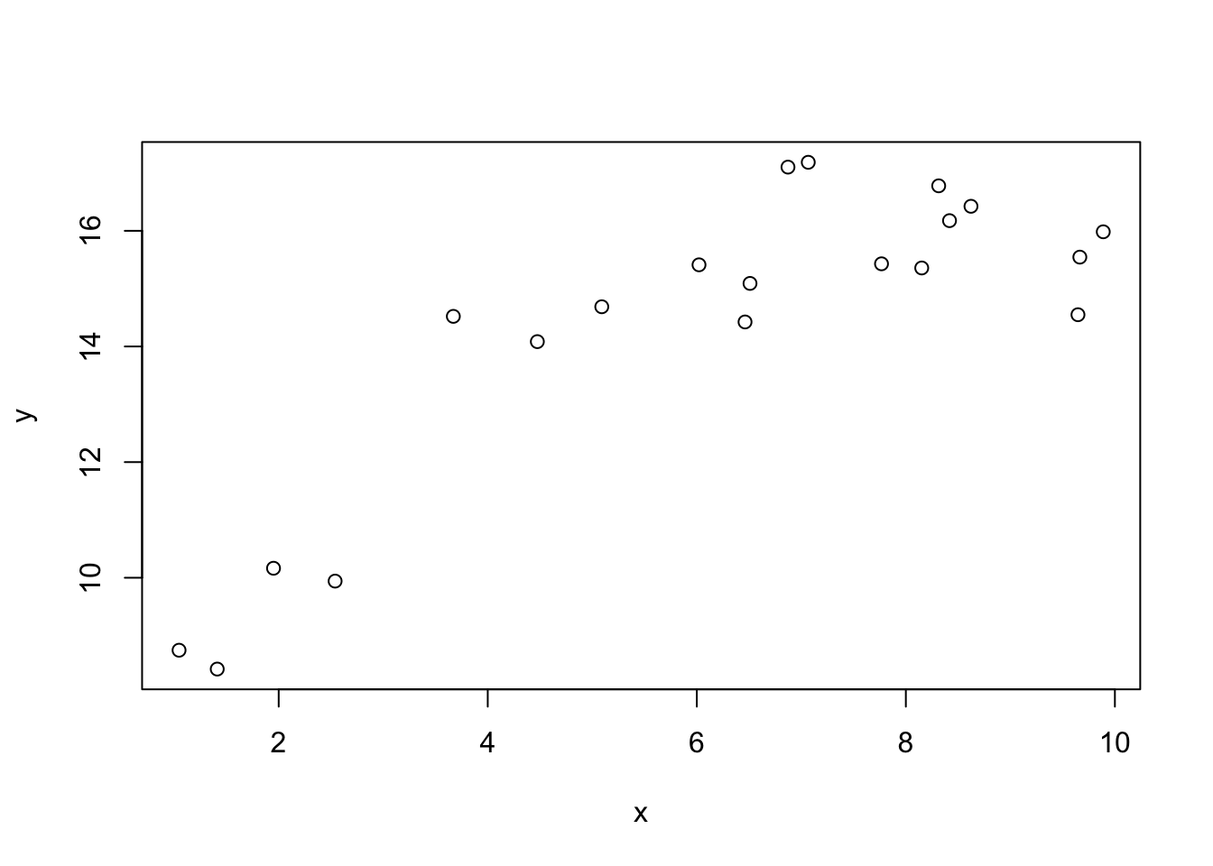
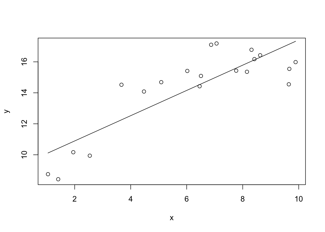
We can fit a linear model to this data and explain some of the variation in y.
Call:
lm(formula = y ~ x)

Residuals:
     Min       1Q   Median       3Q      Max
-2.57936 -1.34904 -0.02879  1.18978  2.26550

Coefficients:
            Estimate Std. Error t value Pr(>|t|)
(Intercept)   9.2619     0.8160  11.351 1.23e-09 ***
x             0.8155     0.1206   6.762 2.46e-06 ***
---
Signif. codes:  0 '***' 0.001 '**' 0.01 '*' 0.05 '.' 0.1 ' ' 1

Residual standard error: 1.487 on 18 degrees of freedom
Multiple R-squared:  0.7175,    Adjusted R-squared:  0.7018
F-statistic: 45.73 on 1 and 18 DF,  p-value: 2.459e-06
We see that x explains about 70% of the variation in y. However looking at the residuals we see evidence for a nonlinear relationship between x and y.
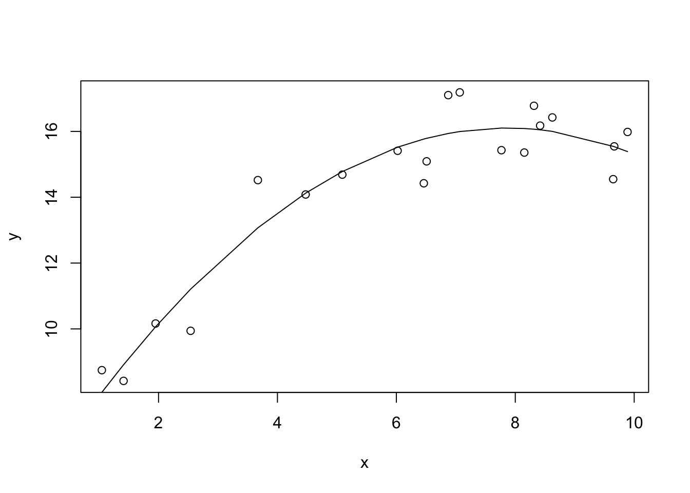
One simple way to account for this would be to add an quadratic term in the model, such that our model is:
\[\hat y = b_0 + b_1 x + b_2 x^2\] We can fit this model in R:
Call:
lm(formula = y ~ x + I(x^2))

Residuals:
     Min       1Q   Median       3Q      Max
-1.34381 -0.67959 -0.01544  0.61630  1.44971

Coefficients:
            Estimate Std. Error t value Pr(>|t|)
(Intercept)  5.41370    0.78967   6.856 2.79e-06 ***
x            2.72222    0.32151   8.467 1.67e-07 ***
I(x^2)      -0.17331    0.02853  -6.075 1.24e-05 ***
---
Signif. codes:  0 '***' 0.001 '**' 0.01 '*' 0.05 '.' 0.1 ' ' 1

Residual standard error: 0.859 on 17 degrees of freedom
Multiple R-squared:  0.9109,    Adjusted R-squared:  0.9004
F-statistic: 86.92 on 2 and 17 DF,  p-value: 1.183e-09
Looking at the coefficients table, we see that the quadratic coefficient is negative, which allows the model to “bend down” at higher values of x, as x^2 becomes >> than x. We also see that this model explains even more variation y (~90%).
If we wanted we can keep adding higher order polynomial terms to our model:
\[\hat y = b_0 + b_1 x + b_2 x^2+ ...+b_n x^n \]
Below I plot out the model predictions for polynomial models as a function of the degree of the polynomial. y ~ x is a first order polynomial with two parameters, y ~ x +x^2 would be a 2nd degree polynomial with three parameters, and so on.
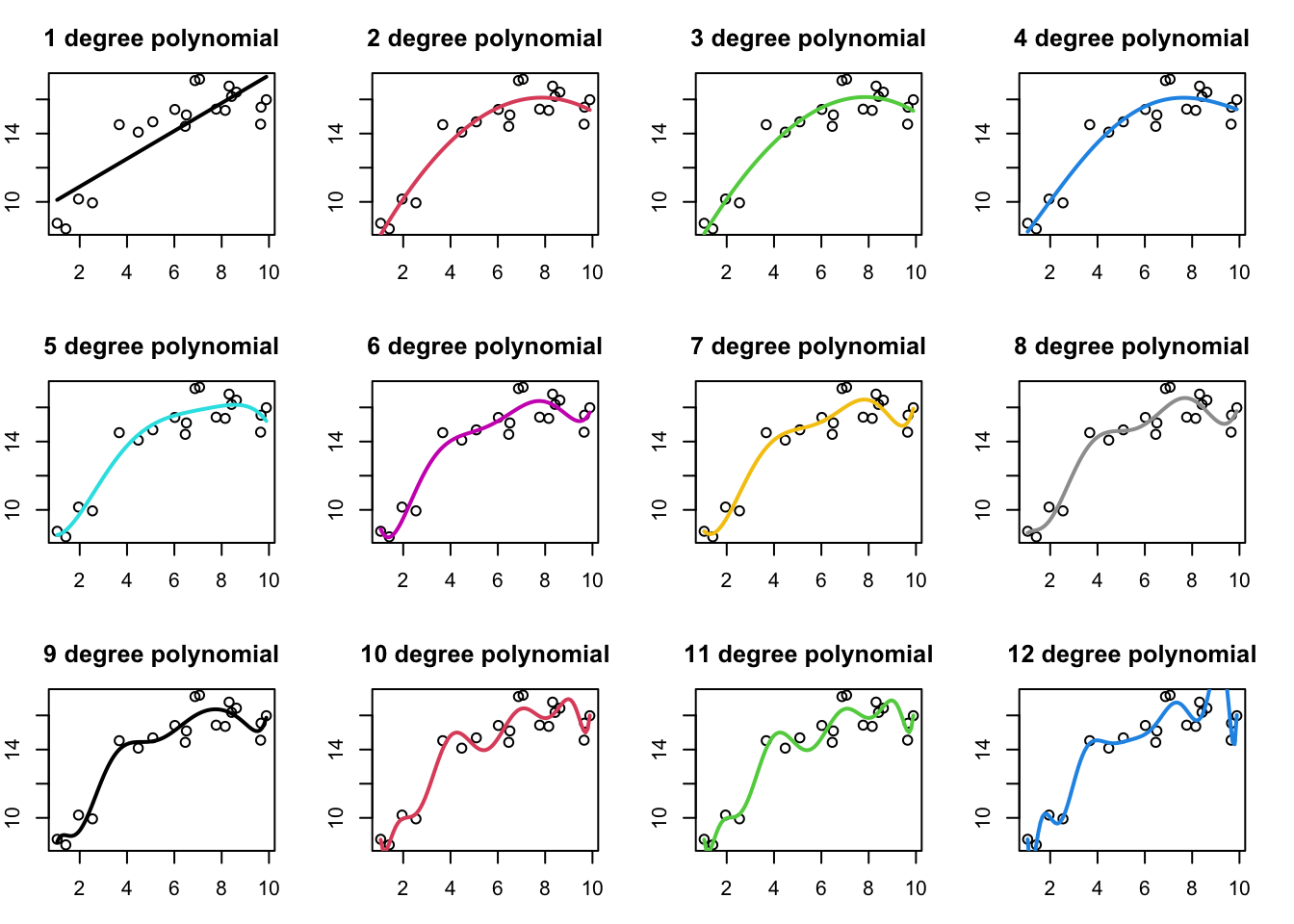
We can see that as our model gets more complex (more fitted parameters), it increasingly does a better job fitting the data, in the sense that the residuals get smaller as we add more terms to the model. Another way to visualize this is to plot out the R^2 as a function of the degree of the polynomial model in the model:
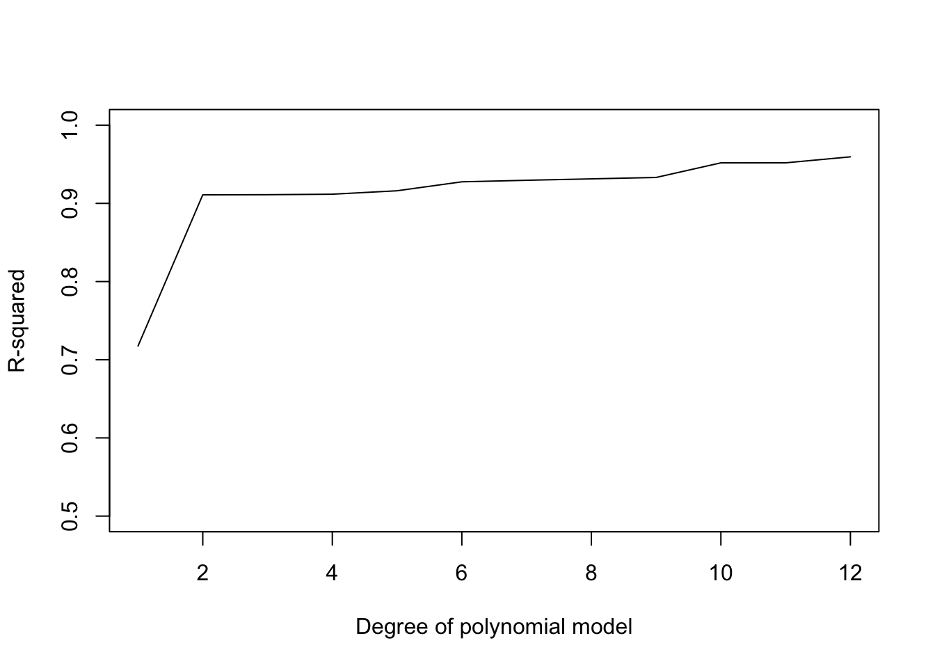
So more complex models will almost always be able to fit our data better. This holds not just for polynomial regression models, but also models with multiple independent variables. Each new variable we add to our model will result in a better model fit (even if only slightly). However, the goal of fitting models to data isn’t to just fit the data we have as well as possible, if that was the goal, we could just draw a line that goes through each data point. You probably already have an intuitive sense the the really complex models (e.g. degree 8 and higher) are perhaps overfitting the data, as the model predictions wiggle up and down to match the data we have as best as possible.
6.2 Cross-validation
While the goals of fitting statistical models are varied (see Advice for model selection), in general, we want our conclusions to generalize to new data. You probably already have an intuitive sense the the really complex models (e.g. degree 8 and higher) are likely overfitting the data we have and would not generalize if we had additional data. One way of assessing the ability of models to generalize to new data sets, is to use some of your data to fit the model, and then leave some of the data out to test the accuracy of the model predictions. This is called cross-validation. There are many different ways to do cross-validation, but one simple version is called leave-one-out-cross-validation (LOOCV). The idea is that we leave out one data point, fit the model to the remaining data, and then evaluate how accurate the prediction was for the observation we left out. This gives us a way of assessing the out-of-sample performance of the model, where out-of-sample, means data the model was not fit with.
We can split out data in R as follows, where I use the sample function to randomly select one observation to be the test observation, or test data, and the remaining data is selected to fit the model (often referred to as the training data)
df<-data.frame(x,y)
test_row = sample(1:length(y),1)
test = df[test_row,]
train =df[-test_row,]
The next step is to fit the model to the training data
mod<-lm(y~x,train)
summary(mod)
Call:
lm(formula = y ~ x, data = train)

Residuals:
    Min      1Q  Median      3Q     Max
-2.4330 -1.1601  0.1000  0.9896  2.1656

Coefficients:
            Estimate Std. Error t value Pr(>|t|)
(Intercept)   9.8691     0.8771   11.25 2.67e-09 ***
x             0.7373     0.1265    5.83 2.01e-05 ***
---
Signif. codes:  0 '***' 0.001 '**' 0.01 '*' 0.05 '.' 0.1 ' ' 1

Residual standard error: 1.431 on 17 degrees of freedom
Multiple R-squared:  0.6666,    Adjusted R-squared:  0.647
F-statistic: 33.99 on 1 and 17 DF,  p-value: 2.009e-05
And then use this model to generate a prediction for the test observation:
mod<-lm(y~x,train)
predict(mod,test)
2
10.91015 If we then compared the predicted value of y against the value of y for the test data, we see that our prediction was off by:
mod<-lm(y~x,train)
test$y - predict(mod,test)
2
-2.489554 We can visualize this by plotting the training data in red, and the test data in blue. The blue vertical line depicts the size of the error for the testing dataset.
df$pred<-predict(mod,df)
test$pred<-predict(mod,test)
ggplot()+geom_point(data=train,aes(x=x,y=y),col='red')+
geom_point(data=test,aes(x=x,y=y),col='blue')+
geom_line(data=df,aes(x=x,y=pred))+
geom_segment(data=test,aes(x=x,xend=x,y=y,yend=pred),col='blue')+
theme_cowplot()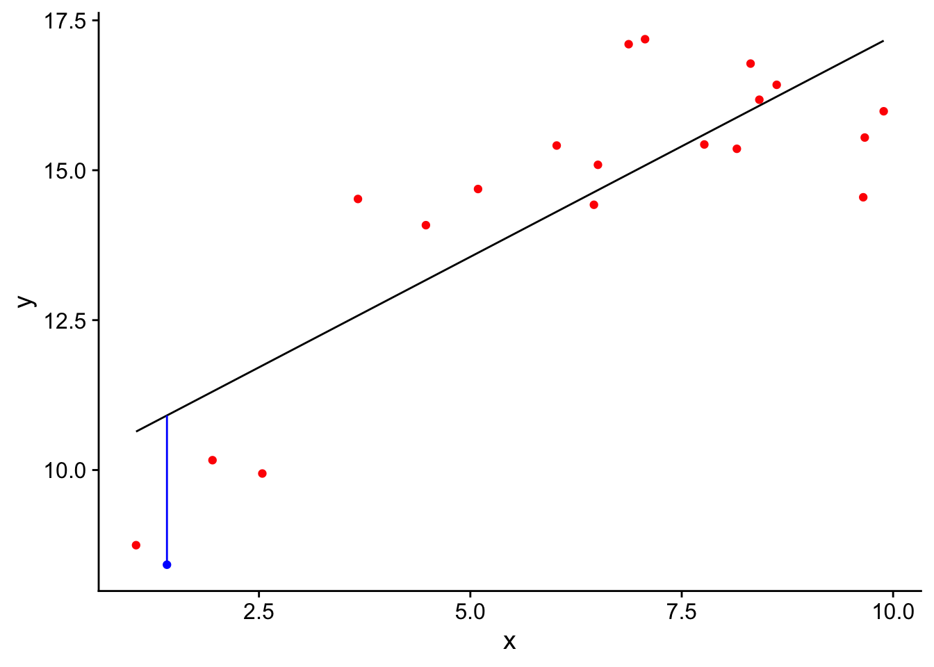 One problem with our method so far is that is our estimate of the prediction accuracy of the model for new data is quite variable, in that it depends a lot on which data point happened to be randomly selected for the test data. One way to reduce this variability is to repeat the analysis once for every data point in our data set. So if we have 20 data points, we fit the model 20 times, each time leaving our one data point of the training set. We can do this with a for loop:
df<-data.frame(x,y)
error<-rep(NA,nrow(df))
for (i in 1:nrow(df)){
  test = df[i,]
  train =df[-i,]
  mod<-lm(y~x,train)
  error[i]<-test$y - predict(mod,test)
}
In the code above, ‘error’ is a vector of the errors for each data point we left out. We can calculate various measures of goodness of fit, for example the standard deviation of the predicted errors:
Pred_SS_Error = sum(error^2)
sqrt(Pred_SS_Error/nrow(df))
[1] 1.591896Or the predicted \(R^2\):
Pred_SS_Error = sum(error^2)
SS_Total = sum((df$y-mean(df$y))^2)
Pred_R2 = 1 - Pred_SS_Error/SS_Total
Pred_R2
[1] 0.640084We can use a nested for loop to repeat this analysis for increasingly complex polynomial models as follows:
Pred_R2<-rep(NA,12)
error<-rep(NA,nrow(df))
PredRMSE<-rep(NA,12)
for (j in 1:12){
  for (i in 1:nrow(df)){
    test = df[i,]
    train =df[-i,]
    mod<-lm(y~poly(x,j),train)
    error[i]<-test$y - predict(mod,test)
  }
  Pred_SS_Error = sum(error^2)
  PredRMSE[j] =  sqrt(Pred_SS_Error/nrow(df))
  Pred_R2[j] = 1 - Pred_SS_Error/SS_Total
}
If we then plot out the predicted R-squared (red line) we see that it peaks at a 2nd degree polynomial model. Furthermore, we see that the predicted R squared drops rapidly for polynomials of degree 8 or higher. This differs form the pattern we found with R^2 on the whole data set that only improved with model complexity (black line).
plot(1:12,Pred_R2,ylim=c(0,1),xlab="Degree of polynomial model",ylab="R-squared",col='red','l')
lines(1:12,R2)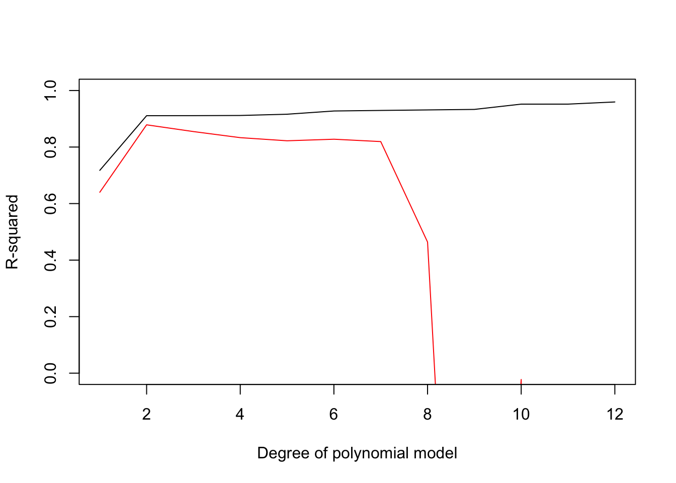 So do we learn from leave-one-out-cross-validation? By repeatedly fitting our model to all but one data point and then testing against the remaining data point, we get a sense for how accurate the prediction of our model would be at predicting a new data point. You probably also noticed that the errors for the test data in LLOCV were larger than for the training data set. This is a very general result. When we assess goodness of fit on data we fit our model to, it will generally overestimate how well it would fit new observations. Thus if you want a more accurate estimate of how accurate your model predictions will be on new data, cross validation is a good choice as the goodness of fit estimates on the training data are generally biased to be to high, especially for models with many parameters.
In some cases, when you are interested in comparing many models, LOOCV can be used as a means of model selection, where models with lower LOOCV error are prefered over models with higher errors.
6.3 AIC
Another way of comparing models is with Akaike information criterion, AIC. The general idea of AIC is that you can compare different models by comparing their likelihood. This is the same likelihood that we used to find the parameters that best fit the data for a specific model with maximum likelihood estimation. We can also use likelihood to compare entirely different models (e.g. different independent variables). In general, when we add more parameters to the model, it will fit the data better, and thus the likelihood will increase as we add more terms. Thus in AIC there is a penalty that we add based on the number of parameters in the model.
AIC = - 2 LL + 2 p
where LL is the log-likelihood and p is the number of parameters in the model. If you remember from chapter 2, the likelihood is the joint probability density of the data given the parameters. To calculate the log-likelihood, we first need to calculate the predicted value of y for each observation, and the residual standard error (our estimate of sigma) for a model. So for the first order polynomial:
  mod<-lm(y~x,df)
  sigma = as.numeric(summary(mod)[6])
  pdf = dnorm(df$y,predict(mod),sigma)
In the code above, pdf is a vector of the probability densities of each observation. They were calculated by providing dnorm() with the observed df$y and predicted predict(mod), values of y, along with the estimate of the standard deviation of the errors, which is the residual standard error (the 6th element of the list of summary(mod)). To calculate the log-likelihood we just need to log the values in pdf, and sum them up. From this we then calculate the AIC score using the formula above:
  p = 2 # intercept and slope
  LL = sum(log(pdf))
  AIC = -2 * LL + 2 * p
  AIC
[1] 74.61517Here we see that the AIC for this model is 74.615, which on its own doesn’t tell us much. Really AIC scores are mostly useful as a relative metric of goodness of fit (releative to other models), with the model with the lowest AIC score being the preferred model. We can rerun the polynomial analysis but calculate AIC scores for each model with the following code:
LL<-rep(NA,12)
AIC<-rep(NA,12)

for (i in 1:12){
  mod<-lm(y~poly(x,i),df)
  sigma = as.numeric(summary(mod)[6])
  LL[i] = sum(log(dnorm(df$y,predict(mod),sigma)))
  AIC[i] = -2*LL[i] + 2*(i+1)
 }
If we plot out the -2 LL and AIC, we see the the negative log-likelihood keeps going down with model complexity (the likelihood goes up), but because of the parameter penalty, the AIC score is minimized at an intermediate complexities (2nd degree polynomial).
plot(1:12,-2*LL,'l',ylab="- 2 log-Likelihood (black) / AIC (red)",xlab="Degree of polynomial")
lines(1:12,AIC,col='red')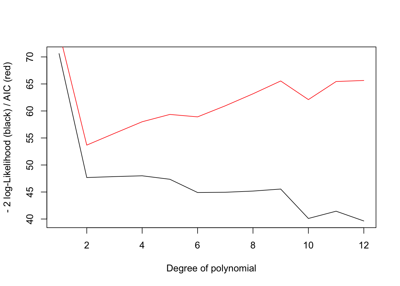
AIC is based off information theory, and AIC estimates the information lost by approximating the real world process that generated the data with a statistical model. The goal is to find the model that minimizes the information lost. We can’t do this with certainty, but AIC seeks to estimate how much more or less information is lost by one model vs another. The relative probability of models losing less information than another can be calculate as:
\[exp((AIC_{min}-AIC_i)/2)\] where \(AIC_{min}\) is the model with the lowest AIC score in the set of models analyzed.
From these relative probabilities you can construct an AIC table, sorted by the AIC score (lowest to highest):
Nparms<-2:13
dfAIC<-data.frame(Nparms)


dfAIC$deltaAIC=min(AIC)-AIC
dfAIC$AICrelLike=exp(dfAIC$deltaAIC/2)
dfAIC$AICweight=dfAIC$AICrelLike/sum(dfAIC$AICrelLike)

dfAIC$AICweight
[1] 1.730573e-05 6.092203e-01 2.052460e-01 7.013522e-02 3.560348e-02 4.460990e-02
[7] 1.602717e-02 5.278258e-03 1.610839e-03 9.020612e-03 1.693373e-03 1.537539e-03dfAICsort <- dfAIC[order(-dfAIC$AICweight),]
dfAICsort<-round(dfAICsort,3)
dfAICsort Nparms deltaAIC AICrelLike AICweight
2 3 0.000 1.000 0.609
3 4 -2.176 0.337 0.205
4 5 -4.324 0.115 0.070
6 7 -5.228 0.073 0.045
5 6 -5.679 0.058 0.036
7 8 -7.276 0.026 0.016
10 11 -8.425 0.015 0.009
8 9 -9.497 0.009 0.005
11 12 -11.771 0.003 0.002
9 10 -11.871 0.003 0.002
12 13 -11.964 0.003 0.002
1 2 -20.938 0.000 0.000The first column indicates the number of paramters. The second column the difference in AIC score between the model with the minimum AIC score and the AIC score that that model (will be zero for the best model). The third column is the relative probability for each model (will be 1 for the best fitting model). The last column is the AIC weight for each model which is calculated by summing up the relative AIC probabilities for all models and dividing the the relative probabilities by the total so that the weights for all models sum to one. Thies weights can be interpreted as the probability a specific model out of all models considered is the model that minimizes information loss.
where \(AIC_{min}\) is the model with the lowest AIC score in the set of models analyzed. We can plot out the relative likelihood of the models as follows:
plot(1:12,dfAIC$AICweight,'l',ylab="AIC weight",xlab="Degree of polynomial")
lines(1:12,AIC,col='red')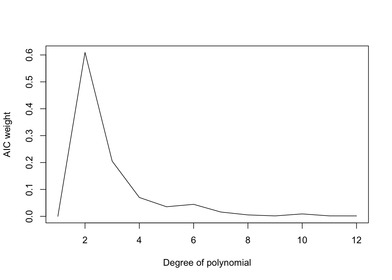 There are other flavors of AIC-like model selection criteria (AICc, BIC). The generally only differ in how large the penalty is for each additional parameter.
We see with the polynomial example, that in terms of model selection, both LOOCV and AIC came to the same conclusion: the model with the lowest LOOCV prediction error also had the lowest AIC score. This will often be the case. I prefer to use LOOCV however because it is based off fewer assumptions and gives you a good estimate of how accurately your model will generate to new data.
In many cases there may be many models that perform roughly equally in either LOOCV or AIC. In these cases, it suggest that different models are roughly equally as consistent with the data, and that more data is needed to differentiate between competting models.
6.4 Advice for model selection
Often when analyzing data we have multiple models or hypotheses that we think could explain a variation in a particular variable and we are interested in comparing how consistent different models are with data. A question you probably have is what is the right way to compare models and select the most likely model or a set of most likely models to focus on. Unfortunately, there is no general answer to this question.
The problem is that we use statistical models for many different purposes (hypothesis testing or inference, data exploration, prediction) and in different contexts (analyzing data from an randomized controlled experiments vs. observational data). For each of these different purposes and contexts we might want to use different strategies to compare models. Below I will outline a couple different contexts we might want to compare models, and what you might want to consider when comparing models.
The only general advice I have about model comparison, is to come up with a plan of how you want to analyze your data before hand. What models do you want to compare? What confounding variables do you think you need to control for? Write down your plan ahead of time, and try to stick to it. If you realize in the middle of analysis that you want to do include a different variable, you can do it, but make sure you record you change your planned and note the reason why you changed your plan. It is good to keep a list of every model that you fit to data, along with the results for each model. When you write up your results, you should also state all the models you tested (and why you tested them). If you looked at a large number of models it may make sense to report the results from all the models in a supplementary table. Such a table might include the a list of which variables were included in the model, the coefficients for each parameter in the model, the standard errors for each coefficient, and one or more metrics of goodness of fit (e.g R^2).
6.4.1 Analysis of experiments
The most straightforward application of model comparisons is for the analysis of randomized controlled experiments. Here we have the advantage that if your experiment was conducted properly, the independent variables should not be correlated with one another. The most common type of experiment that looks at multiple variables, a factorial experimental design. I would generally begin my analysis with the full model that includes each factor and its interaction (at least for a 2-way factorial experiment). If the confidence interval for the parameter associated with the interaction term overlaps with zero, this means that there is a lot of uncertainty about the sign of the interaction given the dataset. In this case it may make sense to look at a simpler model with just the main effects.
6.4.2 Exploratory data analysis
Goal: identify patterns and generate hypotheses
Priority: thoroughly search for patterns
Prior hypothesis: non required
Statistical tools: visualization, correlations, anything goes
Pitfalls: fooling yourself with overfitted models
Sometimes there are many possible variables of interest that might affect your dependent variable. A common example of this is you have data on species abundance or growth rates over time, and then a series of climate variables. For example, you have daily temperature and precipitation data, but only annual estimate of the abundance of some species. You think that it is likely that temperature and precipitation affect the population dynamics of your species, but you aren’t sure exactly which aspect of these variables is most important. For example is it the mean temperature in a year that matters? Or the maximum temperature? Or the minimum temperature? Or is it the variability in temperature? Or the temperature is September? For just this one variable, temperature, we could come up with hundreds of ways to aggregate the variable. In many contexts we find ourselves in the situation where the number of independent variables exceeds the number of data points. The risk with this type of analysis is that if we test many models, there is a good chance we might find a model that fits the data well just due to random chance. It is always important to keep this in mind when you are doing an exploratory analysis: the goal is to identify interesting patterns and generate hypotheses, but finding a strong relationship should not be taken as strong evidence for a hypotheses. Hypothesis testing must be conducted on a independent data set that wasn’t used to generate the hypothesis. Testing hypotheses with the data used to generate them is much like noticing a coincidence, and then assuming it can’t be a coincidence because the odds are too low. For example, it would be like finding out an acquaintance has the same birthday as you, and coming to the conclusion that it can’t be a coincidence, because the probability that you share a birthday is 1/365 which is less than 0.05.
If you want to improve the chances that the patterns identified by an exploratory analysis aren’t spurious, then it is good to limit the models you consider to those that seem plausible. If most of the models you test are implausible, there is a good chance the best models you identify in your analysis with be spurious correlations.
You can use whatever method you like to come up with model in an exploratory analysis. However it is a good idea keep track of how you do the exploratory analysis. For example, one strategy would be to decide on a list of independent variables, then look at the correlation coefficients between each independent variable and the dependent variable and only keep variables with a correlation coefficient above some threshold. Then with this limited set of variables you can look at more complex models (multiple terms or interactions). Alternatively you could use visualization (plots) to try to identify patterns in the data. It is harder to be systemic this way, but at least try to describe the processes of which variables you plotted, and how you went about looking for more complex models.
6.4.3 Inference: Testing hypotheses with observational datasets
Goal: test a hypothesis
Priority: avoid false positives
prior hypothesis: required
statistical tools: parameter estimates, CI, and NHST
pitfalls: doing an exploratory analysis, but then presenting results as a test of a hypothesis
In some cases, we already have a hypothesis or theoretical expectation we wish to test with data. This expectation can either come from a theoretical model or the scientific literature, for example the hypothesis could be based on a pattern identified by a previous exploratory study. In this case, we already have a strong expectation about what we should see in nature, and thus in this case we should really only be testing a very small number of models (ideally just one or two). In general, when our goal is inference, we are asking questions about parameters in our statistical model. For example, we might hypothesize that rainfall is a key variable limiting primary productivity in terrestrial environments, and then our hypothesis is that there should be a positive relationship between rainfall and primary productivity. Or our hypothesis might be that rainfall and sunlight determine primary productivity. In either case, we want to test only a limited set of models. If you can’t limit yourself to a small set of models than you are probably doing an exploitative analysis rather than an inferential analysis.
When you test many different models, reporting a significant result as a test of a hypothesis is problematic because the probability of a false positive is high. If I look at the relationship between primary productivity and 20 different independent variables, chances are I will find a “significant” relationship even if no true relationship exists.
Another thing that is important to keep in mind when testing hypotheses, is whether the data at hand provide a strong test of the hypothesis. For example, say I hypothesized that warmer temperatures were causing a collapse of a threatened fish population, and then fit a statistical model for population growth rate as a function of temperatures and found a significant effect. Is this strong evidence for my original hypothesis? Not necessarily. For example if there are other plausible mechanisms that could have resulted in the collapse of another fish population that are correlated with temperature (overfishing, habitat destruction), then really the data may not necessarily provide strong support for one hypothesis over the other. In this cases, critical thinking is very important. Are there reasonable alternative hypotheses that could explain the trend? If so it is good practice to try to think of other types of data that might discriminate between competing hypotheses, or to try to use experiments to rule out potential explanatory mechanisms.
6.4.4 Robustness checks
With hypotheses testing I personally like to see robustness checks. You have a main hypothesis you want to test using some data set. But in addition to this model, it is useful to check a handful of other reasonable models that could alternatively explain the data. These models should be treated differently then the main hypotheses that are the focus of you analysis, and should not be used for inference, but rather they are a check to see if alternative hypotheses could also explain the pattern you observed. If your original hypothesis compares well against other plausible hypotheses, or the effect you observe is robust to controlling for different variables, this suggest that the result you found is relatively robust, and at least cannot be easily explained by alternative hypotheses. For example my hypothesis is that Y increase with X, but then I also show that alternative hypotheses Y and Z cannot explain variation in Y, this provides additional support to my original hypothesis. Or if I get roughly the same estimated effect of \(X_1\), even after controlling for \(X_2\) and \(X_3\), it suggests the estimate association between \(X_1\) and Y is robust to controlling for other variables of interest.
6.4.5 Null hypothesis tests with large observation datasets are meaningless
Another word of warning related to hypothesis tests with large data sets: If you are analyzing a very large observational data set, there is a good chance that almost any variable would come out as statistically significant on its own. This is because there are generally complex patterns of correlation among variables, and if you have enough data, even small differences among groups will come out as significant. For example, you probably see a headline at least once a week about food X being good or bad for your health. However what we eat is correlated in complex ways with other aspects of our lives: our cultural backgrounds, education, income, etc.. For example if someone looked at a large dataset to test the hypothesis that the risk of getting covid is different for people that drink coffee, vs. don’t drink coffee, they would almost certainly reject the null hypothesis. This probably not because coffee has any causal link to getting Covid, but rather that drinking coffee is associated with many other aspects of our lives that might have some influence of getting Covid. Now, if it turned out that people who drank coffee were much more likely to get covid (e.g. 4 times higher), and the result was robust to many controlling for many potential confounding variables (income, profession, ect.) then it might be worth looking further into whether there is a potential mechanistic link between coffee and Covid. However, if the effect size was relatively small and sensitive to which variables we control for, I wouldn’t take rejecting the null hypothesis as strong eveidence for a link between coffee and Covid.
6.4.6 Prediction
Goal: predict the dependent variable as accurately as possible Priority: minimize prediction error Prior hypothesis: not required, but can be help for picking variables Statistical tools: AIC, out of sample validation pitfalls: failure to validate predictions with out of sample data
Sometimes we just want to be able to predict the value of the dependent variable and we don’t really care about what is in the model so long as it makes accurate predictions. For example, if I was a weather forecaster, I might not care about precisely estimating the relative importance of different independent variables for tomorrows temperature, I just want my forecasts to be as accurate as possible.
When the goal is prediction, analyses begin in a similar way to exploratory analyses. You might want to come up with a list of candidate models you want to test, which can either be based on an exploratory analysis of the data or informed by theory or the literature as to which variables might be useful for predicting the dependent variable of interest. Either AIC or LOOCV can be used for selecting which model to use to make your prediction. However one important difference, is that when your goal is prediction, and you want to truely asses the accuracy of the models predictions, you should leave some faction of the data for an additional level of cross validation. For example, I might use 70% of the data for model selection and leave 30% for testing. On the 70% data I can use either AIC or LOOCV to identify a preferred model that I will use for prediction, and then after I have decided on the model, I can test it’s performance on the remaining 30% of the data. The performance on the out-of-sample data give you an estimate of how well you model might perform on new data. You might think that if you are already doing LOOCV, that you don’t need an additional round of cross-validation. However if you are using LOOCV to compare the performance of a large set of models, the “best” model might have performed well in part due to random chance. So it is a good idea to have an additional level of cross-validation to assess the predictive performance of your model.