5 More complex models
5.1 More than one independent variable
In many cases, we are interested in modeling the dependent variable as a function of more than one independent variable. With general linear models this is easy to incorporate, we just add an additional term in the linear model for each new independent variable. For each new independent variable we also have an additional parameter associated with that variable. All the concepts we applied to single variable models about parameter estimation, standard errors, confidence intervals and hypothesis tests largely apply to more complex models.
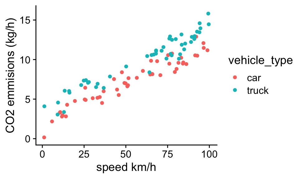
For example, in chapter 1, we introduced a data set for vehicle CO2 emissions that depended on the vehicle type and the speed of travel:
 The simplest linear model we could use to describe this data set would be:
CO2 = b0 + b1 * vehicle_type + b2 * speed
where “vechile_type” is a dummy variable that is 0 for cars and 1 for trucks. We can fit this model to data using the lm function:
mod<-lm(CO2 ~ vehicle_type + speed,df)
summary(mod)
Call:
lm(formula = CO2 ~ vehicle_type + speed, data = df)

Residuals:
     Min       1Q   Median       3Q      Max
-1.95681 -0.51858  0.05663  0.53072  1.99293

Coefficients:
                  Estimate Std. Error t value Pr(>|t|)
(Intercept)       1.954904   0.204214   9.573 1.12e-15 ***
vehicle_typetruck 1.936727   0.176809  10.954  < 2e-16 ***
speed             0.099942   0.003035  32.935  < 2e-16 ***
---
Signif. codes:  0 '***' 0.001 '**' 0.01 '*' 0.05 '.' 0.1 ' ' 1

Residual standard error: 0.8757 on 97 degrees of freedom
Multiple R-squared:  0.9319,    Adjusted R-squared:  0.9305
F-statistic: 664.1 on 2 and 97 DF,  p-value: < 2.2e-16
We can see in the coefficients table above that there are 3 rows of values, with each row corresponding to one of the parameters in our model. For each parameter, we get a parameter estimate, a standard error, a t-value (which is just the estimate divided by the standard error), and a p-value.
Problem 5.1 What is the predicted CO2 emissions of a truck traveling 0 km/h?
At 0 km/h we can ignore the effect of speed. We see that the intercept parameter, \(b_0\) is 1.955 which is the predicted CO2 emissions of cars traveling 0 km/h. The expected difference in CO2 emissions of trucks compared, \(b_1\), to cars is shown in the second row: 1.937. And thus the expected emissions of a truck traveling 0 km/h is \(b_0+b_1\) = 3.892.
Problem 5.2 What is the predicted CO2 emissions of a truck traveling 50 km/h? To answer his question we can just plug in the estimated values of parameters, along with the values of the independent variables we want to make our prediction for into the general linear model equation:
b0 = summary(mod)$coefficients[1,1]
b1 = summary(mod)$coefficients[2,1]
b2 = summary(mod)$coefficients[3,1]

vehicle_type = 1
speed = 50

pred = b0 + b1 * vehicle_type + b2 * speed
pred
[1] 8.888728Problem 5.3 Describe the the estimated effect of speed on CO2 emissions and its uncertainty.
Vehicles traveling 1 km/h faster have an estimated 0.1 kg/h higher emissions. The standard error of this estimate is 0.003, thus we are approximately 95% confident the true population parameter lies between 0.0939 and 0.1059.
Also I didn’t ask for it, but if you were going to do a null hypothesis test, for example, that the population parameter associated with speed = 0, we would see that the estimated parameter value is 33.5 standard errors away from zero (t-value). This alone tells us it would be extremely unlikely to observed this large of a value due to random chance alone (remember 95% of observations are expected to fall within 2 standard errors, and 99.7% within 3 SE). This intuition is confirmed if we look at the very small p-value (less than 2e-16, or 0.00000000000000022), which means we would essentially never see such a strong relationship due to chance alone. It is still important to keep in mind though, especially for observational datasets that just because you have a very low p-value does not imply causation. In this case, a mechanistic link between speed and CO2 emissions is clear, but this won’t always be the case. For example consider the case where fast drivers also listen to loud music. If I fit a model with music volume instead of speed as the independent variable, we would also reject the null hypothesis that the relationship between music volume and CO2 emissions is unlikely to emerge by chance alone. However this would not mean CO2 emissions of a car will directly increase in response to turning the volume up. It is important to remember when analyzing observational data that small p-values doesn’t imply causation, because the observed relationship could always be due to an unmeasured causal variable that is correlated with the independent variable.
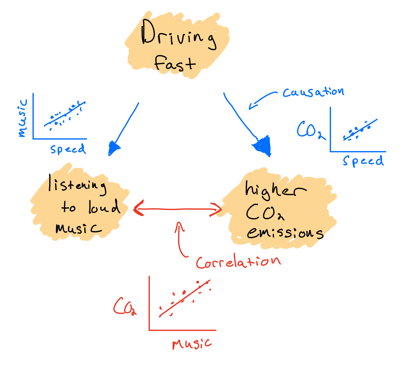
Regression parameters do not necessarily represent causal effects
5.2 Interactions
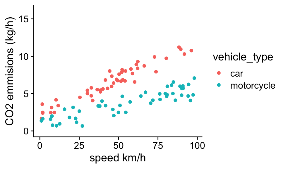
A key assumption of the CO2 emissions model was that the effect of speed on CO2 emissions did not depend on the vehicle type. Looking at the data this seems like a reasonable assumption, but it won’t always be the case. For example, consider a similar dataset, but now comparing the CO2 emissions of cars and motorcycles:
If we repeat the analysis assuming the relationship between speed and emissions is identical for cars and motorcycles:
mod<-lm(CO2 ~ vehicle_type + speed,df)
summary(mod)
Call:
lm(formula = CO2 ~ vehicle_type + speed, data = df)

Residuals:
    Min      1Q  Median      3Q     Max
-4.5741 -0.7047  0.0128  0.7954  1.9902

Coefficients:
                        Estimate Std. Error t value Pr(>|t|)
(Intercept)             3.308149   0.227935   14.51   <2e-16 ***
vehicle_typemotorcycle -3.477201   0.221368  -15.71   <2e-16 ***
speed                   0.069559   0.003825   18.18   <2e-16 ***
---
Signif. codes:  0 '***' 0.001 '**' 0.01 '*' 0.05 '.' 0.1 ' ' 1

Residual standard error: 1.087 on 97 degrees of freedom
Multiple R-squared:  0.834, Adjusted R-squared:  0.8305
F-statistic: 243.6 on 2 and 97 DF,  p-value: < 2.2e-16
We see again a strong association between speed and CO2 emissions, and that motorcycles have lower average CO2 emissions than cars. However, it is also always a good idea to visually inspect the model by plotting out the predictions of the model along with the data. We can do that by creating a new variable in the data frame that contains the predicted value of CO2 emissions for each observation, and then plotting out the model predictions along with the data.
b0 = summary(mod)$coefficients[1,1]
b1 = summary(mod)$coefficients[2,1]
b2 = summary(mod)$coefficients[3,1]

vehicle_type_dummy <- rep(0,nrow(df))
vehicle_type_dummy[df$vehicle_type == "motorcycle"] = 1
df$prediction<- b0 + b1* vehicle_type_dummy + b2* df$speed


ggplot(df,aes(x=speed,y=CO2,group=vehicle_type))+
  geom_point(aes(color=vehicle_type))+
  geom_line(aes(x=speed,y=prediction,color=vehicle_type))+
  theme_cowplot()+ylim(0,16)+xlab("speed km/h")+ylab("CO2 emmisions (kg/h)")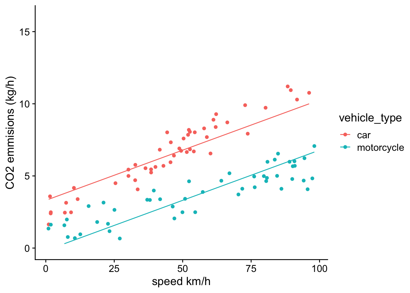
While the model fit looks pretty good, if you inspect carefully, you see that the residuals tends to show systematic bias. For example, for cars, most observed CO2 emissions are lower than the predicted value at low speeds, and above the predicted value at high speeds. The opposite pattern is true for motorcycles. This suggest that the relationship between CO2 emissions and speed might differ for cars vs. motorcycles. In statistical models, when the effect of one independent variable depends on the value of another independent variable, we call it an interaction, or an interactive effect.
In general we can add an interaction in our statistical model by creating a new state variable that is the product of two independent variables:
\[\hat y = b_0 + b_1 x_1 + b_2 x_2 + b_3 x_1 x_2 \] where \(b_3\) captures the effect of the interaction.
Problem 5.3 Going back to the emissions example, lets assume \(x_1\) is the dummy variables that is 0 for cars and 1 for motorcycles, and \(x_2\) is speed. Based on this you should be able to work out the interpretation of each of parameter in the model. Hint: plug in the value of the dummy variable into the equation and remove terms that equal zero.
We can get the formula for cars by setting \(x_1\) to 0, which eliminates the 2nd and 4th term in the linear model, such that: \[\hat y (cars)= b_0 + b_2 x_2 \] From this we can see that \(b_0\) is the expected CO2 emissions for cars at 0 km/h, and \(b_2\) is the rate of increase in CO2 emissions with speed for cars.
We now have interpretations for two of the parameters in our linear model. We can identify the interpretation of the remaining two, but setting \(x_1\) to 1, which results in:
\[\hat y (motorcycles)= b_0 + b_1 + (b_2 + b_3) x_2 \] We can see that when speed is 0, the predicted CO2 emissions of motorcycles is \(b_0 +b_1\). Remembering the the predicted CO2 emissions of cars at 0 km/h is \(b_0\), we can see that \(b_1\) is the expected difference in emissions for motorcycles vs. cars at 0 km/hr. Similarly, we can see that emissions increase by \(b_2 +b_3\) for each unit increase in speed for motorcycles. Because emissions increase by \(b_2\) per unit speed for cars, we can interpret the parameter \(b_3\) as the expected difference in slope of CO2 emissions with speed in motorcycles vs. cars.
We can fit a model with an interaction using the lm() function as follows:
mod<-lm(CO2 ~  vehicle_type + speed + vehicle_type:speed,df)
summary(mod)
Call:
lm(formula = CO2 ~ vehicle_type + speed + vehicle_type:speed,
    data = df)

Residuals:
    Min      1Q  Median      3Q     Max
-3.3638 -0.5290  0.0588  0.5942  1.6177

Coefficients:
                              Estimate Std. Error t value Pr(>|t|)
(Intercept)                   1.997425   0.244763   8.161 1.30e-12 ***
vehicle_typemotorcycle       -1.145352   0.344293  -3.327  0.00125 **
speed                         0.099353   0.004841  20.523  < 2e-16 ***
vehicle_typemotorcycle:speed -0.048403   0.006170  -7.844 6.05e-12 ***
---
Signif. codes:  0 '***' 0.001 '**' 0.01 '*' 0.05 '.' 0.1 ' ' 1

Residual standard error: 0.853 on 96 degrees of freedom
Multiple R-squared:  0.8988,    Adjusted R-squared:  0.8957
F-statistic: 284.3 on 3 and 96 DF,  p-value: < 2.2e-16
Problem 5.4 What is the estimated rate of increase of CO2 emissions with speed for motorcycles?
The last row in the coefficient table represents the estimated difference in the slope of CO2 emissions with speed for motorcycles vs. cars. We see that this value is negative which suggests that the rate of increase of CO2 emissions for motorcycles is lower than for cars, and based on the values of \(b_2\) and \(b_3\), would be approximately: 0.051.
We also can see that the standard error for the interaction parameter is small relative to the estimated value. This suggest that a model with different slopes for CO2 as a function speed for cars and motorcycles is more consistent with the data than a model that assumes the slopes are identical: \(b_3=0\).
Finally, we can evaluate the fit of the model by plotting out its predictions along with the data:
b0 = summary(mod)$coefficients[1,1]
b1 = summary(mod)$coefficients[2,1]
b2 = summary(mod)$coefficients[3,1]
b3 = summary(mod)$coefficients[4,1]
vehicle_type_dummy <- rep(0,nrow(df))
vehicle_type_dummy[df$vehicle_type == "motorcycle"] = 1
df$prediction<- b0 + b1* vehicle_type_dummy + b2* df$speed +b3 * df$speed * vehicle_type_dummy
ggplot(df,aes(x=speed,y=CO2,group=vehicle_type))+
geom_point(aes(color=vehicle_type))+
geom_line(aes(x=speed,y=prediction,color=vehicle_type))+
theme_cowplot()+ylim(0,16)+xlab("speed km/h")+ylab("CO2 emmisions (kg/h)")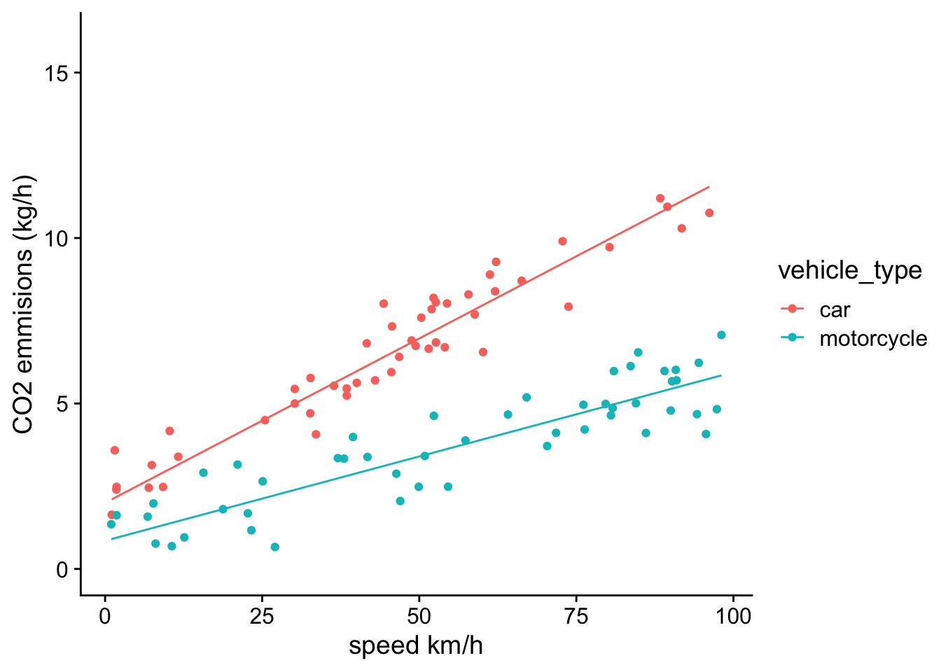 Visually inspecting this model reveals that the residuals are no longer systemically biased as a function of speed. This further suggests that a model with an interaction term makes sense in this case.
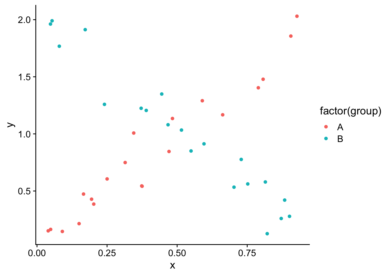
One important thing to keep in mind is that you need to be careful interpreting the main effect of individual variables when there is an interaction. This is because the “effect” of one independent variable depends on the value of the other independent variable. For example if we had the following data:
 And we fit a linear model:
summary(lm(y~group*x,df))
Call:
lm(formula = y ~ group * x, data = df)

Residuals:
     Min       1Q   Median       3Q      Max
-0.29079 -0.09822  0.01382  0.10375  0.30066

Coefficients:
            Estimate Std. Error t value Pr(>|t|)
(Intercept)  0.04117    0.05863   0.702    0.487
groupB       1.97709    0.09059  21.825   <2e-16 ***
x            1.92891    0.11846  16.283   <2e-16 ***
groupB:x    -3.87844    0.16625 -23.329   <2e-16 ***
---
Signif. codes:  0 '***' 0.001 '**' 0.01 '*' 0.05 '.' 0.1 ' ' 1

Residual standard error: 0.1474 on 36 degrees of freedom
Multiple R-squared:  0.9394,    Adjusted R-squared:  0.9344
F-statistic: 186.1 on 3 and 36 DF,  p-value: < 2.2e-16
We see that the main effect of group B is positive (~2), which if there was no interaction would suggest that the value of y for group B is ~2 units higher that group A for a given level of x. However because there is a strong interaction, we can see in the plot that whether group B has a higher value of y than A depends on x. The interpretation of the main parameter is the estimated difference between B vs. A when x = 0. In general, when you have an interaction it is useful to plot out the predictions of the model to interpret model parameters:
mod<-(lm(y~group*x,df))
df$pred  <-predict(mod)
ggplot(df,aes(x=x,y=y,group=group))+
  geom_point(aes(col=factor(group)))+
  geom_line(aes(x=x,y=pred,col=factor(group)))+theme_cowplot()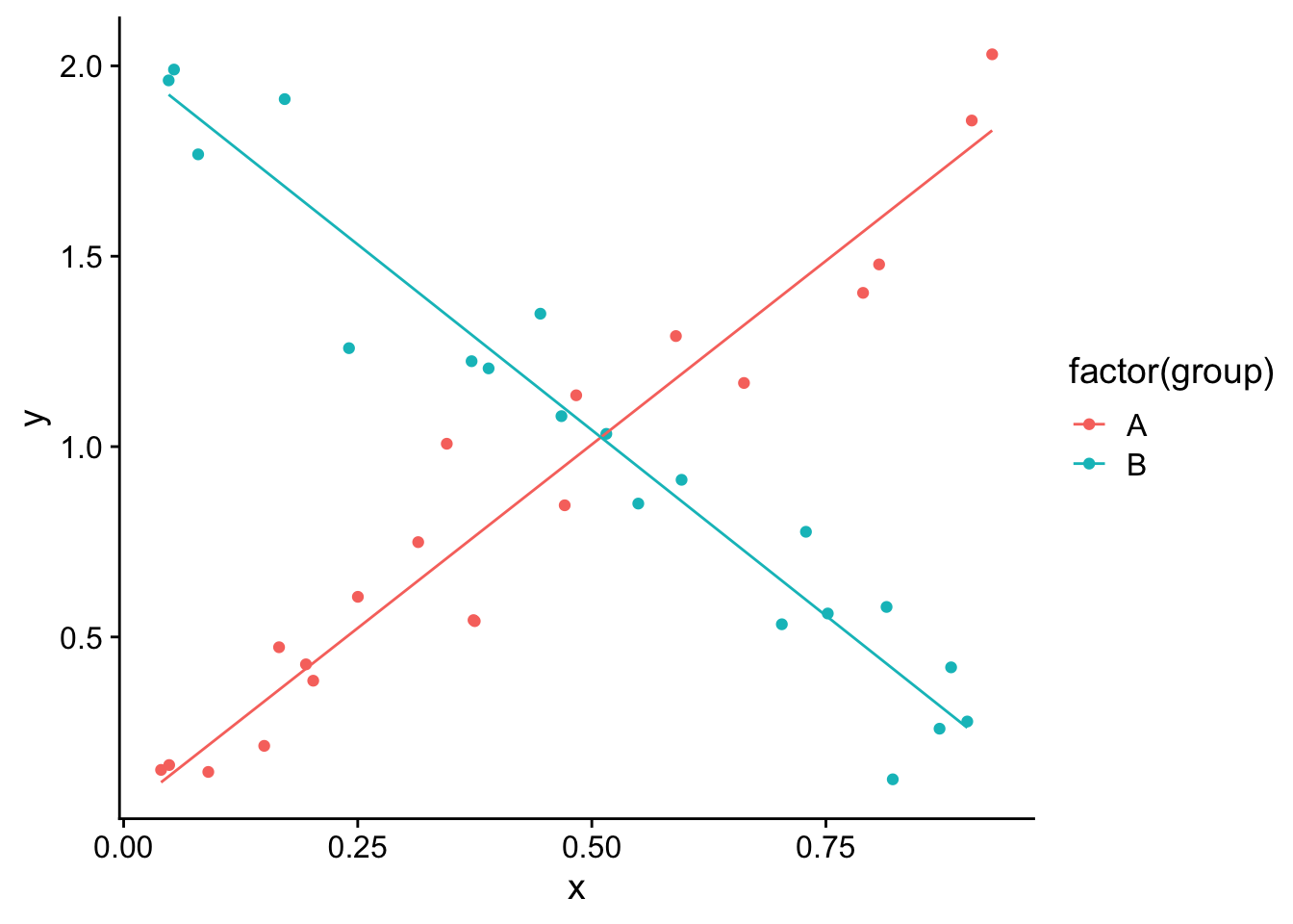
In this case we can see that the predicted value of y for each group depends on x. When x is 0, group B has a higher value of y, but the predicted value of y decreases with x for group B, while it increases with x for group A. Thus at higher values of x, group A has a higher predicted value of y than group B.
5.3 Controlling for a variable
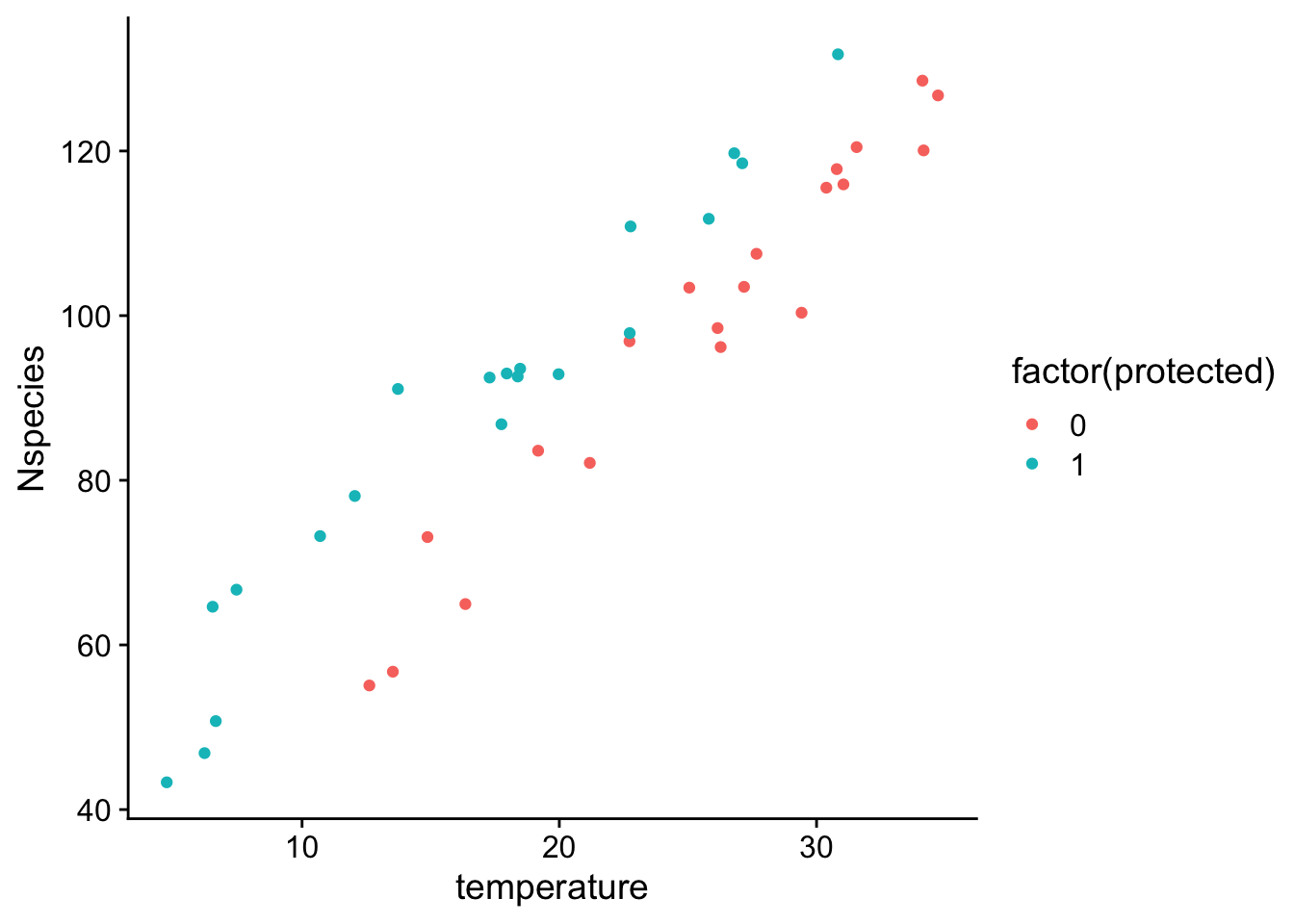
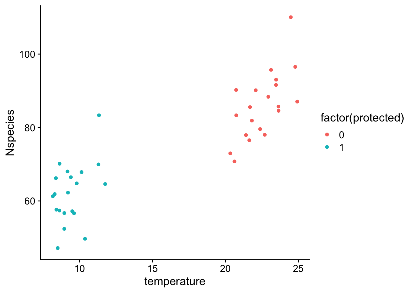
Sometimes our hypothesis is related to the importance of a specific independent variable, but we know that other variables have strong impacts on the dependent variable. For example, we might be interested in whether there are more species of insects in protected (no industry and logging) forests vs. unprotected forests, but we also know that there tends to be more insects in warmer areas. Our primary interest is in the difference between protected and unprotected forests, but we think another variable (temperature) will cause a lot of variation in the dependent variable. If we don’t account for this variable, it can 1) cause there to be a high residual error and thus high standard error of parameter estimates, and 2) if the level of the control variable is not balanced among the variable of interest (e.g. more protected forests in warmer locations) then it can lead to biased parameter estimates (e.g. because there is some correlation between protection status and temperature. If we don’t account for temperature, the influence of temperature will show up in the estimated affects of protection status).
Here we I illustrate these points with the following data:
 If we just fit a model with only the variable of interest (protection status):
mod<-lm(Nspecies~protected,df)
summary(mod)
Call:
lm(formula = Nspecies ~ protected, data = df)

Residuals:
    Min      1Q  Median      3Q     Max
-44.512 -15.129   4.721  18.056  43.924

Coefficients:
            Estimate Std. Error t value Pr(>|t|)
(Intercept)   98.352      5.282   18.62   <2e-16 ***
protected    -10.530      7.470   -1.41    0.167
---
Signif. codes:  0 '***' 0.001 '**' 0.01 '*' 0.05 '.' 0.1 ' ' 1

Residual standard error: 23.62 on 38 degrees of freedom
Multiple R-squared:  0.04969,   Adjusted R-squared:  0.02468
F-statistic: 1.987 on 1 and 38 DF,  p-value: 0.1668
We see first that the estimated effect of protecting a forest is negative (reduces the number of species), and second that there is a relatively large standard error for the parameter estimate. If we remember from Chapter 3 that the standard error of parameter estimates increases in proportion to the standard deviation of the residuals, it makes sense that our estimates of parameter values are imprecise.
However if we re-run the analysis with temperature in the model to account for variation in the number of species in an area due to temperature:
mod<-lm(Nspecies~protected+temperature,df)
summary(mod)
Call:
lm(formula = Nspecies ~ protected + temperature, data = df)

Residuals:
    Min      1Q  Median      3Q     Max
-10.152  -4.352   0.367   3.675  12.367

Coefficients:
            Estimate Std. Error t value Pr(>|t|)
(Intercept)  20.4147     3.2089   6.362 2.04e-07 ***
protected    16.2712     1.9928   8.165 8.45e-10 ***
temperature   3.0625     0.1168  26.223  < 2e-16 ***
---
Signif. codes:  0 '***' 0.001 '**' 0.01 '*' 0.05 '.' 0.1 ' ' 1

Residual standard error: 5.41 on 37 degrees of freedom
Multiple R-squared:  0.9515,    Adjusted R-squared:  0.9489
F-statistic: 362.8 on 2 and 37 DF,  p-value: < 2.2e-16
Problem 5.5 We now see the estimated number of species is higher in protected vs. unprotected forests as opposed to being lower when temperature was not included in the model. Why caused this difference?
In this case we can see from the plot that there is a bit of correlation between temperature and protected status, in that temperatures in protected forests tended to be cooler on average than unprotected forests. Because forests with cooler temperatures also tend to have less species, when we fit a model without temperature, we actually estimated that protected forests have fewer species.
Problem 5.6 We can also see that the standard error associated with the effect of protection status is now much lower now that we have included temperature in the model. Why did including temperature as a independent variable reduce the the standard error for the parameter associated with protection status?
Because temperature appears to explain a large amount of variation in the number of species present in forests, including it in the statistical model reduced the standard residual error. Because standard errors of parameter estimates increase with the standard residual error, reducing the errors allows model parameters to be estimated more precisely.
In summary, we often want to control for variables to 1) reduce the residual errors and consequently increase the precision in our parameter estimates and 2) avoid bias in our estimates of parameters of interest that may occur when there is some correlation between our independent variable of interest and confounding variables.
5.4 Multicollinearity
The correlation between protected status and temperature was mild in the last example, in that there was still a fair amount of overlap in temperatures between protected and unprotected forests. However in other cases, the correlation can be more extreme. For example, if the data looked like this:
we now see that there is much stronger correlation between protection status and temperature. All the forests that are protected are from cooler climates than unprotected forests. The problem this creates is that it becomes difficult to estimate the parameters in the model because variation in the dependent variable could be attributed to either independent variable. For example, if we fit a model with either temperature or protection status alone, we would find strong associations for each independent variable:
Protection status model:
mod_protect<-lm(Nspecies~protected,df)
summary(mod_protect)
Call:
lm(formula = Nspecies ~ protected, data = df)

Residuals:
     Min       1Q   Median       3Q      Max
-15.2060  -5.3933  -0.2404   4.6935  24.0627

Coefficients:
            Estimate Std. Error t value Pr(>|t|)
(Intercept)   85.972      1.948  44.125  < 2e-16 ***
protected    -23.896      2.755  -8.672 1.53e-10 ***
---
Signif. codes:  0 '***' 0.001 '**' 0.01 '*' 0.05 '.' 0.1 ' ' 1

Residual standard error: 8.713 on 38 degrees of freedom
Multiple R-squared:  0.6643,    Adjusted R-squared:  0.6555
F-statistic: 75.21 on 1 and 38 DF,  p-value: 1.53e-10
Temperature model:
mod_temp<-lm(Nspecies~temperature,df)
summary(mod_temp)
Call:
lm(formula = Nspecies ~ temperature, data = df)

Residuals:
     Min       1Q   Median       3Q      Max
-13.7106  -4.7581   0.4887   4.8336  19.9009

Coefficients:
            Estimate Std. Error t value Pr(>|t|)
(Intercept)  43.7757     3.1365   13.96  < 2e-16 ***
temperature   1.8932     0.1812   10.45 9.89e-13 ***
---
Signif. codes:  0 '***' 0.001 '**' 0.01 '*' 0.05 '.' 0.1 ' ' 1

Residual standard error: 7.641 on 38 degrees of freedom
Multiple R-squared:  0.7419,    Adjusted R-squared:  0.7351
F-statistic: 109.2 on 1 and 38 DF,  p-value: 9.892e-13
But if we include a model with both variables:
mod_temp<-lm(Nspecies~ protected+ temperature,df)
summary(mod_temp)
Call:
lm(formula = Nspecies ~ protected + temperature, data = df)

Residuals:
     Min       1Q   Median       3Q      Max
-16.1107  -5.7975   0.6444   4.2684  16.3863

Coefficients:
            Estimate Std. Error t value Pr(>|t|)
(Intercept)  -2.5923    21.2914  -0.122 0.903753
protected    27.6398    12.5660   2.200 0.034163 *
temperature   3.9303     0.9421   4.172 0.000175 ***
---
Signif. codes:  0 '***' 0.001 '**' 0.01 '*' 0.05 '.' 0.1 ' ' 1

Residual standard error: 7.282 on 37 degrees of freedom
Multiple R-squared:  0.7717,    Adjusted R-squared:  0.7594
F-statistic: 62.54 on 2 and 37 DF,  p-value: 1.354e-12
We see that both terms are “statistically significant” but that there are quite large standard errors, especially for the parameter associated with protection status. In this case, even through both variables come out as “statistically significant” the data available probably is not sufficient to test the hypothesis that protected forests have more species than unprotected forests. This is because our linear model makes a lot of assumptions that are hard to asses. For example, our model assumes that the relationship between temperature and the number of species is the same for protected and unprotected areas, but given that the temperatures in protected and unprotected forests do not overlap, it is really difficult to asses this assumption. Our model also assumes the affect of temperature is linear, but because we only have a limited range of temperatures within each type of forest it is difficult to assess this assumption. Thus this is a case where even though the results of the statistical test are significant common sense and critical thinking suggests that we should be very cautious about interpreting the results of this test.
When two or more independent variables are highly correlated, we call this multicollinearity. Multicollinearity is very common in observational data sets, especially in ecological time series. The general problem is that when independent variables are highly correlated, it can be difficult to estimate the effects of individual independent variables. For example, consider that case where you doctor tells you that you need to improve your health, and prescribes you some medication. At the same time, you start eating better, and getting more regular sleep. After a few weeks you health improves. The question is, did you health improve because of the medication? Or eating better? Or getting more regular sleep? Or some combination of the three? In this example, it is difficult to tell because the 3 potential explanatory variables were all correlated. This is exactly the same problem when we have correlated independent variables, multicollinearity makes it hard to assess the relative importance of the independent variables. As a result when we fit models with correlated independent variables, the standard errors of the parameter estimates tend to be large. The more correlated the variables, the larger the standard errors will be for the parameters associated with those variables.
If we are trying to test hypotheses about the relative importance of two independent variables for some dependent variable of interest, and the two independent variables are highly correlated, then if we include both terms in the model, the standard errors of the parameter estimates will likely be large and perhaps overlap zero (the parameter associated with the independent variable could be positive or negative). In this case the data are not really sufficient to test our hypothesis, because there is not enough independent variation in the independent variables to be able to assess whether the dependent variable is more strongly associated with one or the other independent variable. In this case, the best option is to try to find more data (or do an experiment) where the independent variables are not correlated.
Sometimes our goal is prediction rather than inference. In this case we don’t care as much about the parameter estimates, but rather how accurately our model predicts the dependent variable. In this case, multicollinearity is not problematic, because it generally does not affect the predictive performance of linear models (e.g. the residual standard error).
5.5 What you should know
1. How to write down equations for linear models with multiple independent variables
2. How to fit linear models with multiple independent variables or control variables, and interpret the output of models
3. Understand and interpret interactive effects in statistical models
5. Understand what multicollinearity is, and how it affects the conclusions we can draw from analyses