5. Regression Discontinuity
Key Concepts
- Regression discontinuity is used to estimate the effect of a program when the following conditions are met:
- There is a discrete cut-off (e.g. score, poverty index, class size) that divides the sample into treatment and control groups.
- The cut-off is based on a continuous rather than categorical variable.
- Regression discontinuity provides esitmates for those around the cut-off score, not observations far from it.
- It answers questions such as "should the program be cut or expanded at the margin?
Methods Matter, Chapter 9
The following example comes from Murnane and Willett (2010), chapter 9.
Maimonides’ Rule and the Impact of Class Size on Student Achievement
This data looks at a natural experiment in Israel in which class sizes must be split if they exceed 40 students, making those over 20+, and, thus, smaller class sizes.
# load packages
library(tidyverse)
library(haven)
library(gt)
library(janitor)
library(apaTables)
source("data/apafunction.R")Note: observations are at the classroom-level
Variables:
- read: verbal score (class average)
- size: average class cohort size during September enrollment
- intended_classize: average intended class size for each school
- observed_classize: average actual size for each school
Descriptives
as_tibble(psych::describe(class_size), rownames = "variable") %>%
  mutate(across(where(is.numeric), round, 3)) %>%
    select(variable, n, mean, sd, min, max) %>%
apa()| variable | n | mean | sd | min | max |
|---|---|---|---|---|---|
| read | 2019 | 74.379 | 7.678 | 34.8 | 93.86 |
| size | 2019 | 77.742 | 38.811 | 8.0 | 226.00 |
| intended_classize | 2019 | 30.956 | 6.108 | 8.0 | 40.00 |
| observed_classize | 2019 | 29.935 | 6.546 | 8.0 | 44.00 |
Box plots of classrooms within analytic window
class_size %>%
  filter(between(size, 36, 46)) %>%
  ggplot()+
  geom_boxplot(aes(x=as.factor(size), y=read))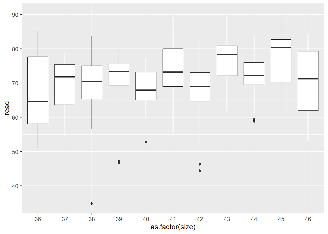
class_size %>%
  filter(between(size, 36, 46)) %>%
  group_by(size) %>%
  summarize(freq = n(),
            mean_intended = mean(intended_classize, na.rm=T),
            mean_observed = mean(observed_classize, na.rm=T),
            mean_read = mean(read, na.rm=T),
            sd_read = sd(read, na.rm = T)) %>%
apa("Table 9.1 on page 168")| Table 9.1 on page 168 | |||||
|---|---|---|---|---|---|
| size | freq | mean_intended | mean_observed | mean_read | sd_read |
| 36 | 9 | 36.0 | 27.44444 | 67.30445 | 12.363886 |
| 37 | 9 | 37.0 | 26.22222 | 68.94066 | 8.497514 |
| 38 | 10 | 38.0 | 33.10000 | 67.85400 | 14.038258 |
| 39 | 10 | 39.0 | 31.20000 | 68.87000 | 12.072376 |
| 40 | 9 | 40.0 | 29.88889 | 67.92847 | 7.865053 |
| 41 | 28 | 20.5 | 22.67857 | 73.67670 | 8.766867 |
| 42 | 25 | 21.0 | 23.40000 | 67.59560 | 9.302938 |
| 43 | 24 | 21.5 | 22.12500 | 77.17644 | 7.466089 |
| 44 | 17 | 22.0 | 24.41176 | 72.16160 | 7.712399 |
| 45 | 19 | 22.5 | 22.73684 | 76.91684 | 8.708218 |
| 46 | 20 | 23.0 | 22.55000 | 70.30814 | 9.783913 |
Difference Analysis for 40/41 Class Size
Difference analysis discussed on page 172.
Create cut-off groups
T-test of small (0) and large (1) class sizes
class_ttest1 <- class_size %>%
  filter(size == 40 | size == 41)
t.test(class_ttest1$read ~ class_ttest1$small, var.equal = T) %>%
  broom::tidy() %>%
  mutate(across(is.numeric, round, 3)) %>%
  rename("small class" = estimate1,
         "large class" = estimate2) %>%
apa("T-test for class sizes of 40 or 41")| T-test for class sizes of 40 or 41 | ||||||||
|---|---|---|---|---|---|---|---|---|
| small class | large class | statistic | p.value | parameter | conf.low | conf.high | method | alternative |
| 67.928 | 73.677 | -1.751 | 0.089 | 35 | -12.414 | 0.918 | Two Sample t-test | two.sided |
Interpretation
This t-test compare class sizes of only 40 students in the small class size group and 41 in the large class size group. The results show that large classes (with 41 students) had higher mean scores, but this result was not statistically significant.
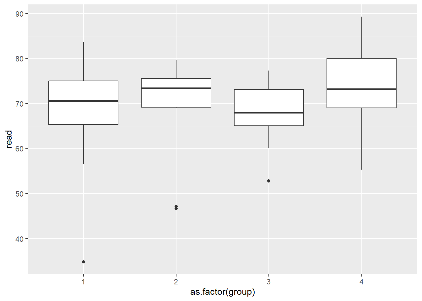
Difference Analaysis of Four Class Sizes
Difference analysis discussed starting on page 173. (Output not shown in text.)
class_four <- class_size %>%
  filter(size>=38 & size<=41) %>%
  mutate(group = case_when(
    size == 38 ~ 1,
    size == 39 ~ 2,
    size == 40 ~ 3,
    size == 41 ~ 4
  ))

class_four %>%
  group_by(group) %>%
  summarize(N = n(),
            mean = mean(read),
            variance = var(read)) %>%
  mutate(across(where(is.numeric), round, 3)) %>%
apa()| group | N | mean | variance |
|---|---|---|---|
| 1 | 10 | 67.854 | 197.073 |
| 2 | 10 | 68.870 | 145.742 |
| 3 | 9 | 67.928 | 61.859 |
| 4 | 28 | 73.677 | 76.858 |
Setup for RDD Regression
“larger” distinguishes the group with the larger enrollment in any pair.
“first” distinguishes the groups that participate in the first diff.
predictors <- class_four %>%
  mutate(larger = ifelse(group == 2 | group == 4, 1, 0),
         first = ifelse(group == 3 | group == 4, 1, 0))

rdd_model1 <- lm(read ~ first+larger+first*larger, data=predictors)

apa.reg.table(rdd_model1)[[3]] %>%
apa()| Predictor | b | b_95%_CI | sr2 | sr2_95%_CI | Fit |
|---|---|---|---|---|---|
| (Intercept) | 67.85** | [61.30, 74.41] | |||
| first | 0.07 | [-9.45, 9.59] | .00 | [-.00, .00] | |
| larger | 1.02 | [-8.25, 10.28] | .00 | [-.01, .02] | |
| first:larger | 4.73 | [-7.47, 16.93] | .01 | [-.04, .06] | |
| R2 = .071 | |||||
| 95% CI[.00,.19] | |||||
| Predictor | SS | df | MS | F | p | partial_eta2 | CI_90_partial_eta2 |
|---|---|---|---|---|---|---|---|
| (Intercept) | 46041.65 | 1 | 46041.65 | 431.48 | .000 | ||
| first | 0.03 | 1 | 0.03 | 0.00 | .988 | .00 | [.00, 1.00] |
| larger | 5.16 | 1 | 5.16 | 0.05 | .827 | .00 | [.00, .04] |
| first x larger | 64.57 | 1 | 64.57 | 0.61 | .440 | .01 | [.00, .10] |
| Error | 5655.37 | 53 | 106.71 | ||||
fig91_data <- class_size %>%
  mutate(group = case_when(
    size == 36 ~ 1,
    size == 37 ~ 2,
    size == 38 ~ 3,
    size == 39 ~ 4,
    size == 40 ~ 5,
    size == 41 ~ 6
  )) %>%
  drop_na(group) %>%
  group_by(group) %>%
  summarize(mread = mean(read))

fig91_data %>%
  filter(group != 6) %>%
  ggplot()+
  geom_point(aes(x=as.factor(group),
                y=mread))+
  geom_line(aes(x=group,
                y=mread))+
  geom_smooth(aes(x=group,
                y=mread), method='lm', se=F)+
  geom_point(data=(fig91_data %>%
               filter(group == 6)),
             aes(x=as.factor(group),
                y=mread))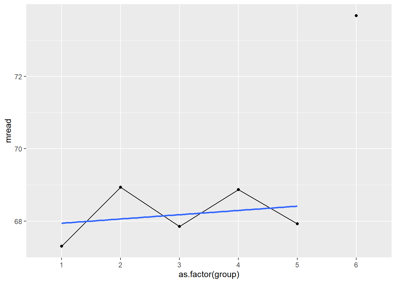
Actual RDD
Table 9.3 on page 180.
rdd_data <- class_size %>%
  mutate(small = ifelse(size<=40, 0, 1),
         csize = size-41)

# RDD estimate for size between 36 and 46
rdd_model2 <- lm(read ~ csize + small, data=rdd_data %>%
                   filter(between(size, 36, 46)))

apa.reg.table(rdd_model2)[[3]] %>%
apa("Regression-discontinuity estimate of the impact of an offer of small versus large classes on class-average reading achievement, using data from classes in the fifth-grade enrollment cohorts of size 36 through 41 in Israeli Jewish public schools")| Regression-discontinuity estimate of the impact of an offer of small versus large classes on class-average reading achievement, using data from classes in the fifth-grade enrollment cohorts of size 36 through 41 in Israeli Jewish public schools | ||||||||
|---|---|---|---|---|---|---|---|---|
| Predictor | b | b_95%_CI | beta | beta_95%_CI | sr2 | sr2_95%_CI | r | Fit |
| (Intercept) | 68.70** | [64.91, 72.48] | ||||||
| csize | 0.17 | [-0.69, 1.03] | 0.05 | [-0.20, 0.30] | .00 | [-.01, .01] | .19* | |
| small | 3.85 | [-1.70, 9.40] | 0.17 | [-0.08, 0.42] | .01 | [-.02, .04] | .21** | |
| R2 = .046* | ||||||||
| 95% CI[.00,.11] | ||||||||
Interpretation
- intercept: Reading score for schools at the 41 cutoff.
- csize: A one-unit change in class size is associated with a .17 reading score increase
- small: the causal effect of interest
- Larger classes are associated with a 3.85 score increase
RDD Analytic Window Variations
rdd_model3 <- lm(read ~ csize + small, data=rdd_data %>%
                   filter(between(size, 36, 41)))

rdd_model4 <- lm(read ~ csize + small, data=rdd_data %>%
                   filter(between(size, 35, 47)))

rdd_model5 <- lm(read ~ csize + small, data=rdd_data %>%
                   filter(between(size, 34, 48)))

rdd_model6 <- lm(read ~ csize + small, data=rdd_data %>%
                   filter(between(size, 33, 49)))

rdd_model7 <- lm(read ~ csize + small, data=rdd_data %>%
                   filter(between(size, 32, 50)))

rdd_model8 <- lm(read ~ csize + small, data=rdd_data %>%
                   filter(between(size, 31, 51)))

rdd_model9 <- lm(read ~ csize + small, data=rdd_data %>%
                   filter(between(size, 30, 52)))

rdd_model10 <- lm(read ~ csize + small, data=rdd_data %>%
                   filter(between(size, 29, 53)))

tribble(
  ~Window, ~csize, ~csize_p, ~small, ~small_p, ~r2, ~MS,
  "36-46",
    rdd_model2[["coefficients"]][["csize"]],
    summary(rdd_model2)$coefficients[2,4],
    rdd_model2[["coefficients"]][["small"]],
    summary(rdd_model2)$coefficients[3,4],
    summary(rdd_model2)$r.squared,
    apa.aov.table(rdd_model2)[["table_body"]][["MS"]][4],
  "36-41",
    rdd_model3[["coefficients"]][["csize"]],
    summary(rdd_model3)$coefficients[2,4],
    rdd_model3[["coefficients"]][["small"]],
    summary(rdd_model3)$coefficients[3,4],
    summary(rdd_model3)$r.squared,
    apa.aov.table(rdd_model3)[["table_body"]][["MS"]][4],
  "35-47",
    rdd_model4[["coefficients"]][["csize"]],
    summary(rdd_model4)$coefficients[2,4],
    rdd_model4[["coefficients"]][["small"]],
    summary(rdd_model4)$coefficients[3,4],
    summary(rdd_model4)$r.squared,
    apa.aov.table(rdd_model4)[["table_body"]][["MS"]][4],
  "34-48",
    rdd_model5[["coefficients"]][["csize"]],
    summary(rdd_model5)$coefficients[2,4],
    rdd_model5[["coefficients"]][["small"]],
    summary(rdd_model5)$coefficients[3,4],
    summary(rdd_model5)$r.squared,
    apa.aov.table(rdd_model5)[["table_body"]][["MS"]][4],
  "33-49",
    rdd_model6[["coefficients"]][["csize"]],
    summary(rdd_model6)$coefficients[2,4],
    rdd_model6[["coefficients"]][["small"]],
    summary(rdd_model6)$coefficients[3,4],
    summary(rdd_model6)$r.squared,
    apa.aov.table(rdd_model6)[["table_body"]][["MS"]][4],
  "32-50",
    rdd_model7[["coefficients"]][["csize"]],
    summary(rdd_model7)$coefficients[2,4],
    rdd_model7[["coefficients"]][["small"]],
    summary(rdd_model7)$coefficients[3,4],
    summary(rdd_model7)$r.squared,
    apa.aov.table(rdd_model7)[["table_body"]][["MS"]][4],
  "31-51",
    rdd_model8[["coefficients"]][["csize"]],
    summary(rdd_model8)$coefficients[2,4],
    rdd_model8[["coefficients"]][["small"]],
    summary(rdd_model8)$coefficients[3,4],
    summary(rdd_model8)$r.squared,
    apa.aov.table(rdd_model8)[["table_body"]][["MS"]][4],
  "30-52",
    rdd_model9[["coefficients"]][["csize"]],
    summary(rdd_model9)$coefficients[2,4],
    rdd_model9[["coefficients"]][["small"]],
    summary(rdd_model9)$coefficients[3,4],
    summary(rdd_model9)$r.squared,
    apa.aov.table(rdd_model9)[["table_body"]][["MS"]][4],
  "29-53",
    rdd_model10[["coefficients"]][["csize"]],
    summary(rdd_model10)$coefficients[2,4],
    rdd_model10[["coefficients"]][["small"]],
    summary(rdd_model10)$coefficients[3,4],
    summary(rdd_model10)$r.squared,
    apa.aov.table(rdd_model10)[["table_body"]][["MS"]][4]
) %>%
  mutate(across(where(is.numeric), round, 3)) %>%
apa("Comparison of models at different analytics windows - key statistics selected")| Comparison of models at different analytics windows - key statistics selected | ||||||
|---|---|---|---|---|---|---|
| Window | csize | csize_p | small | small_p | r2 | MS |
| 36-46 | 0.171 | 0.696 | 3.847 | 0.173 | 0.046 | 93.58 |
| 36-41 | 0.124 | 0.908 | 5.120 | 0.205 | 0.066 | 103.79 |
| 35-47 | 0.017 | 0.957 | 4.122 | 0.101 | 0.037 | 90.34 |
| 34-48 | 0.002 | 0.994 | 4.012 | 0.083 | 0.036 | 86.87 |
| 33-49 | -0.013 | 0.951 | 3.672 | 0.090 | 0.030 | 83.43 |
| 32-50 | 0.028 | 0.878 | 2.966 | 0.147 | 0.025 | 81.21 |
| 31-51 | 0.036 | 0.816 | 2.927 | 0.133 | 0.026 | 83.04 |
| 30-52 | -0.044 | 0.741 | 3.362 | 0.069 | 0.020 | 80.93 |
| 29-53 | -0.139 | 0.243 | 3.953 | 0.029 | 0.015 | 84.30 |
Impact Evaluation, Chapter 6
This example compares health expenditures at follow-up between households just above and just below the poverty index threshold, in the treatment localities.
“We start by normalizing the poverty index threshold to 0 and create dummy variables for households with a poverty-targeting index to the left or right of the threshold. By doing so, we allow the relationship between the outcome variables and the running variable (the poverty index) to have different slopes on either side of the threshold. We then run a regression of health expenditures on a dummy variable capturing exposure to the program, as well as the two dummies for whether households have a poverty index to the left or to the right of the threshold” (p. 27)
impact_rdd <- read_dta("data/impact_evaluation/evaluation.dta") %>%
  # select treatment localities
  filter(treatment_locality==1) %>%
  # Normalize the poverty index:
  mutate(poverty_index_left = ifelse(
            poverty_index<=58,
            poverty_index-58,
            0),
         poverty_index_right = ifelse(
           poverty_index>58,
           poverty_index-58,
           0
         ))

impact_rdd_model1 <- lm(health_expenditures ~ poverty_index_left+
      poverty_index_right + eligible, data=impact_rdd %>%
        filter(round ==1))


apa.reg.table(impact_rdd_model1)[[3]] %>%
  apa("RDD example from page 27")
| RDD example from page 27 | ||||||||
|---|---|---|---|---|---|---|---|---|
| Predictor | b | b_95%_CI | beta | beta_95%_CI | sr2 | sr2_95%_CI | r | Fit |
| (Intercept) | 20.55** | [19.89, 21.22] | ||||||
| poverty_index_left | 0.18** | [0.12, 0.23] | 0.09 | [0.06, 0.12] | .00 | [.00, .01] | .43** | |
| poverty_index_right | 0.22** | [0.16, 0.28] | 0.11 | [0.08, 0.14] | .01 | [.00, .01] | .43** | |
| eligible | -11.19** | [-12.11, -10.28] | -0.44 | [-0.48, -0.41] | .08 | [.06, .09] | -.57** | |
| R2 = .338** | ||||||||
| 95% CI[.32,.36] | ||||||||
Additional resource:
https://evalf19.classes.andrewheiss.com/class/10-class/#slides
Related Journal Articles
Bleemer, Z., & Mehta, A. (2020). Will studying economics make you rich? A regression discontinuity analysis of the returns to college major.
Zhang, L., Hu, S., Sun, L., & Pu, S. (2016). The effect of Florida’s Bright Futures Program on college choice: A regression discontinuity approach. The Journal of Higher Education, 87(1), 115-146.
References
Gertler, P. J., Martinez, S., Premand, P., Rawlings, L. B., & Vermeersch, C. M. (2016). Impact evaluation in practice. The World Bank.
Murnane, R. J., & Willett, J. B. (2010). Methods matter: Improving causal inference in educational and social science research. Oxford University Press.