4. Difference-in-Differences

Key Concepts

• Discontinuity Design - A research measures the treatment effect when a forcing variable such as time, a natural disaster, or policy change “randomly” places individuals into treatment and control groups and establishes a clear cut-point for these groups.
• Difference-in-Differences - A design that is useful when a relationship between an outcome and the forcing variable may exist
  • This means that there are differences in the groups that may affect the outcome between groups

Methods Matter, Chapter 8

The following example comes from Murnane and Willett (2010), chapter 8.

Social Security Survivor Benefits

A “natural experiment” looking at college attendance outcome of those before and after 1981. “In 1981, the U.S. Congress eliminated the SSSB program, mandating that otherwise eligible children who were not enrolled in college as of May 1982 would not receive” financial aid that they were previously entitled to.

# load packages
library(tidyverse)
library(haven)
library(gt)
library(janitor)
source("data/apafunction.R")

#load and prep data
sssb <- read_dta("data/methods_matter/ch8_dynarski.dta") %>%
  mutate(fatherdec = as_factor(fatherdec))

Variables:

• id: individual ID?
• hhid: ?
• wt88: sampling weights
• coll: enrolled full-time in college by age 23 (1=yes | 0=no)
• hgc23: highest grade completed by age 23 (10-19)
• yearsr: year in which a senior
• fatherdec: father deceased by age 18 (1=yes | 0=no)
• offer: senior in year SSSB support available (1=yes | 0=no)

Survey Data and Weights

The survey contains weighted data and therefore must be treated differently from typical data frames. Here, survey weighting and setup can be accomplished with either survey or srvyr packages. They are quite similar, and, indeed, sryvr is used in conjunction with survey. The primary difference is that srvyr can be used with tidyverse dplyr verbs such as mutate() and summarize().

First examples are given using both packages.

survey package instructions come from https://stylizeddata.com/how-to-use-survey-weights-in-r/

srvyr package instructions come from https://cran.r-project.org/web/packages/srvyr/vignettes/srvyr-vs-survey.html

library(survey)
library(srvyr)


# using `survey`
survey_data <- svydesign(id      = ~hhid,
                          weights = ~wt88,
                          nest    = F,
                          data    = sssb)

# using `srvyr`
srvy_data <- sssb %>% as_survey_design(ids = hhid, 
                              weights = wt88)

Descriptive statistics

Survey: Mean estimation

# using `survey`
svymean(~coll, survey_data) %>%
  knitr::kable()

	mean	coll
coll	0.4943504	0.0105154

# using `srvyr`
srvy_data %>%
  summarize(mean = survey_mean(coll)) %>%
  apa()

mean	mean_se
0.4943504	0.01051536

Interpretation

About 49% of students enrolled in college.

Cross tabulation of “fatherdec” by “yearsr”

sssb %>%
  tabyl(fatherdec, yearsr) %>% # cross tab
  adorn_totals("row") %>% # make a total row
  rowwise() %>% # perform a mutation across rows
  mutate(Total = sum(`79`,`80`,`81`,`82`,`83`)) %>% # sum rows
  apa() %>%
   tab_spanner(
    label = "Year in which a senior",
    columns = vars(`79`,`80`,`81`,`82`,`83`)
   )

fatherdec	Year in which a senior					Total
	79	80	81	82	83
Father not deceased	892	986	867	828	222	3795
Father deceased	41	44	52	41	13	191
Total	933	1030	919	869	235	3986

Direct Estimate

Estimate means

# mean estimation by levels

# using `srvyr`
srvy_data %>%
  group_by(fatherdec, offer) %>% 
  summarize(means = survey_mean(coll)) %>%
  apa("Direct Estimate shown in Table 8.1 on page 143 using srvyr")

Direct Estimate shown in Table 8.1 on page 143 using srvyr
fatherdec	offer	means	means_se
Father not deceased	0	0.4756935	0.01886493
Father not deceased	1	0.5017016	0.01217353
Father deceased	0	0.3522178	0.08124455
Father deceased	1	0.5604556	0.05274389

Estimate first difference by t-test

# select only "father deceased"
direct_subset <- srvy_data %>%
  filter(fatherdec == "Father deceased")

# t-test with `survey` function
svyttest(coll~offer, direct_subset) %>%
  broom::tidy() %>%
  apa()

estimate	statistic	p.value	parameter	conf.low	conf.high	method	alternative
0.2082378	2.233214	0.02683979	170	0.02547938	0.3909962	Design-based t-test	two.sided

Interpretation

Those who in the pre-1981 cohort (those whose father was deceased and who had recieved an offer of support for college) had a 21 percentage point higher enrollment than those in the post-1981 cohort (deceased father with no offer of support). Note that this is the first difference and is not a valid final interpretation because of possibly innate differences between the groups. Thus, we need a second difference. (See Murnane et al., 2010, p. 154)

Estimate t-test by hand

# calculate t value from table above
(0.5604556-0.3522178)/sqrt(0.05274389^2 + 0.08124455^2)

## [1] 2.1498

# p-value from one-sided test
# from https://www.cyclismo.org/tutorial/R/pValues.html#calculating-a-single-p-value-from-a-t-distribution

pt(-abs(2.1498),df=191-1)

## [1] 0.01641762

Direct Estimate / First Difference (via OLS)

# model
srvy_ols <- svyglm(coll ~ offer,
          family = gaussian(),
          data   = srvy_data,
          design = direct_subset)

# make a table
broom::tidy(srvy_ols) %>%
  mutate(across(is.numeric, round, 3)) %>%
  add_row(term = "r2",
           estimate = poliscidata::fit.svyglm(srvy_ols, 
                                               digits = 3)) %>%
            slice(-4) %>%
  apa("Linear-Probability Model (OLS) Estimate shown in Table 8.1 on page 143")%>%
  fmt_missing(
    columns = 2:5,
    missing_text = ""
  )

Linear-Probability Model (OLS) Estimate shown in Table 8.1 on page 143
term	estimate	std.error	statistic	p.value
(Intercept)	0.352	0.081	4.335	0.000
offer	0.208	0.093	2.233	0.027
r2	0.036

Interpretation is the same as the t-test above

Graph of data

# it is easier to make a graph via `srvyr`, `dplyr` verbs, and `ggplot`
srvy_data %>%
  group_by(fatherdec, offer) %>% 
  summarize(means = survey_mean(coll)) %>%
  ungroup() %>%
  mutate(offer = dplyr::recode(offer,
                        `1` = "Pre-1981", 
                        `0` = "Post-1981")) %>%
  ggplot()+
  geom_line(aes(x=fct_rev(offer), y=means, group=1))+
  facet_wrap(~fct_rev(fatherdec))+
  scale_y_continuous(limits=c(0,1))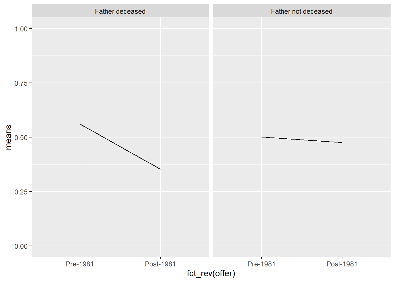

Second Difference

# select only "father NOT deceased"
srvy_subset2 <- srvy_data %>%
  filter(fatherdec == "Father not deceased")

# model
srvy_ols2 <- svyglm(coll ~ offer,
          family = gaussian(),
          data   = srvy_data,
          design = srvy_subset2)

# make a table
broom::tidy(srvy_ols2) %>%
  mutate(across(is.numeric, round, 3)) %>%
  add_row(term = "r2",
           estimate = poliscidata::fit.svyglm(srvy_ols2, 
                                               digits = 3)) %>%
            slice(-4) %>%
  apa("Table 8.2 on page 157, labeled (Second Diff)")%>%
  fmt_missing(
    columns = 2:5,
    missing_text = ""
  )

Table 8.2 on page 157, labeled (Second Diff)
term	estimate	std.error	statistic	p.value
(Intercept)	0.476	0.019	25.216	0.000
offer	0.026	0.021	1.223	0.221
r2	0.001

Interpretation

This model of second difference includes only those whose fathers were not decreased and thus models the trend of this group (the counterfactual group) and its enrollment trend, which had a modest decline of 3 percentage points.

Full Difference-in-Differences Model

# model
srvy_did <- svyglm(coll ~ offer + fatherdec + offer*fatherdec,
          family = gaussian(),
          data   = srvy_data,
          design = srvy_data)

# make a table
broom::tidy(srvy_did) %>%
  mutate(across(is.numeric, round, 3)) %>%
  add_row(term = "r2",
           estimate = poliscidata::fit.svyglm(srvy_did, 
                                               digits = 3)) %>%
  slice(-6) %>%
  apa("Table 8.4 on page 161.")%>%
  fmt_missing(
    columns = 2:5,
    missing_text = ""
  )

Table 8.4 on page 161.
term	estimate	std.error	statistic	p.value
(Intercept)	0.476	0.019	25.216	0.000
offer	0.026	0.021	1.223	0.221
fatherdecFather deceased	-0.123	0.083	-1.480	0.139
offer:fatherdecFather deceased	0.182	0.096	1.901	0.057
r2	0.002

Interpretation

This interaction of offer x father deceased indicates our difference-in-differences estimate, which means that those who recieved an offer of support and whose fathers were decreased had higher enrollment than those who did not recieve financial support with decreased fathers.

Impact Evaluation, Chapter 7

The following example comes from Gertler, Martinez, Premand, Rawlings, and Vermeersch (2016), chapter 8. Data is from The World Bank. The example below is from Stata Example 8. Difference-in-Differences in a Regression Framework, page 22, of the Impct Evaluation Technical Companion.

# load packages
library(tidyverse)
library(haven)
library(gt)
library(janitor)
library(apaTables)
source("data/apafunction.R")

Health Expenditures

In this method, you compare the change in health expenditures over time between enrolled and nonenrolled households in the treatment localities.

#load and prep data
impact_data <- read_dta("data/impact_evaluation/evaluation.dta")

Difference-in-Differences in a Regression Framework

impact_did <- lm(health_expenditures ~ round + eligible + eligible*round, data=impact_data %>%
                 filter(treatment_locality == 1)) %>%
  apa.reg.table()

apa(impact_did$table_body, impact_did$table_title)

Regression results using health_expenditures as the criterion
Predictor	b	b_95%_CI	sr2	sr2_95%_CI	Fit
(Intercept)	20.79**	[20.44, 21.14]
round	1.51**	[1.02, 2.00]	.00	[.00, .00]
eligible	-6.30**	[-6.75, -5.85]	.05	[.04, .06]
round:eligible	-8.16**	[-8.80, -7.53]	.04	[.04, .05]
					R2 = .344**
					95% CI[.33,.36]

Interpretation

This model indicates a difference-in-differences estimate of US$8.16 lower health expenditures for those eligible to be enrolled in this program (eligible) in the follow-up period (round i.e., survey round).

Difference-in-Differences in a Multivariate Regression Framework

impact_did2 <- lm(health_expenditures ~ round*eligible + ., data =
                    impact_data %>%
                    filter(treatment_locality == 1) %>%
                    dplyr::select(health_expenditures, round, eligible, age_hh, age_sp, educ_hh, educ_sp, female_hh, indigenous, hhsize, dirtfloor, bathroom, land, hospital_distance)) %>%
  apa.reg.table()

apa(impact_did2$table_body, impact_did2$table_title)

Regression results using health_expenditures as the criterion
Predictor	b	b_95%_CI	sr2	sr2_95%_CI	Fit
(Intercept)	27.39**	[26.49, 28.30]
round	1.45**	[1.04, 1.86]	.00	[.00, .00]
eligible	-1.51**	[-1.92, -1.10]	.00	[.00, .00]
age_hh	0.08**	[0.06, 0.10]	.00	[.00, .01]
age_sp	-0.02*	[-0.04, -0.00]	.00	[-.00, .00]
educ_hh	0.06*	[0.00, 0.12]	.00	[-.00, .00]
educ_sp	-0.08*	[-0.14, -0.01]	.00	[-.00, .00]
female_hh	1.10**	[0.63, 1.58]	.00	[.00, .00]
indigenous	-2.31**	[-2.60, -2.02]	.01	[.01, .01]
hhsize	-1.99**	[-2.06, -1.93]	.17	[.15, .18]
dirtfloor	-2.30**	[-2.58, -2.01]	.01	[.01, .01]
bathroom	0.50**	[0.23, 0.77]	.00	[-.00, .00]
land	0.09**	[0.05, 0.13]	.00	[.00, .00]
hospital_distance	-0.00	[-0.01, 0.00]	.00	[-.00, .00]
round:eligible	-8.16**	[-8.69, -7.64]	.04	[.04, .05]
					R2 = .552**
					95% CI[.54,.56]

Interpretation

This model has the same interpretation as above, only it includes many more statistical controls. Note that the DD estimate is actually slightly lower past the second decimal place. Note also the higher \(R^2\).

---

Related Journal Articles

Cornwell, C., & Mustard, D. B. (2006). Merit aid and sorting: The effects of HOPE-style scholarships on college ability stratification. IZA Discussion Paper No. 1956.

Furquim, F., Corral, D., & Hillman, N. (2020). A Primer for Interpreting and Designing Difference-in-Differences Studies in Higher Education Research. Higher Education: Handbook of Theory and Research: Volume 35, 667-723.

References

Gertler, P. J., Martinez, S., Premand, P., Rawlings, L. B., & Vermeersch, C. M. (2016). Impact evaluation in practice. The World Bank.

Murnane, R. J., & Willett, J. B. (2010). Methods matter: Improving causal inference in educational and social science research. Oxford University Press.